

A data science interview will include a variety of challenging questions asking you to utilize your skills in machine learning, probability, SQL and more. Don’t be intimidated by the length of this guide. I’ve broken it down into four, manageable sections to help you prepare: machine learning, probability, SQL and miscellaneous.
10 Data Science Interview Questions to Practice
- What are some of the steps for data wrangling and data cleaning before applying machine learning algorithms?
- How do you deal with unbalanced binary classification?
- What Is the difference between a boxplot and a histogram?
- Describe different regularization methods, such as L1 and L2 regularization?
- If the probability that an item at location A is 0.6 and 0.8 at location B, what is the probability that the item would be found on Amazon?
- Explain the difference between convex and non-convex cost functions. What does it mean When a cost function is non-convex?
- Walk through the fundamentals of probability.
- Write a SQL query to get the second highest salary from an employee table.
- If there are 8 Marbles of equal weight and 1 marble that’s a little heavier for a total of 9 marbles, how many weighings does it take to determine which marble is heaviest?
- Define quality assurance and six sigma.
Think of this as a workbook or a crash course filled with tens of data science interview questions that you can use to hone your knowledge and to identify gaps that you can then fill afterwards.
Data Science Interview Questions: Machine Learning
1. What Are Some of the Steps for Data Wrangling and Data Cleaning Before Applying Machine Learning Algorithms?
There are many steps that can be taken when data wrangling and data cleaning. Some of the most common steps include:
- Data profiling: Almost everyone starts off by getting an understanding of their data set. More specifically, you can look at the shape of the data set with .shape and a description of your numerical variables with
.describe(). - Data visualizations: Sometimes, it’s useful to visualize your data with histograms, boxplots and scatterplots to better understand the relationships between variables and also to identify potential outliers.
- Syntax error: This includes making sure there’s no white space, making sure letter casing is consistent, and checking for typos. You can check for typos by using
.unique()or by using bar graphs. - Standardization or normalization: Depending on the data set you’re working with and the machine learning method you decide to use, it may be useful to standardize or normalize your data so that different scales of different variables don’t negatively impact the performance of your model.
- Handling null values: There are a number of ways to handle null values including deleting rows with null values altogether, replacing null values with the mean/median/mode, replacing null values with a new category (i.e., unknown), predicting the values, or using machine learning models that can deal with null values.
- Other things to consider: Removing irrelevant data, removing duplicates and type conversion.
2. How Do You Deal With Unbalanced Binary Classification?
There are a number of ways to handle unbalanced binary classification, assuming that you want to identify the minority class:
- First, you want to reconsider the metrics that you’d use to evaluate your model. The accuracy of your model might not be the best metric to look at,and I’ll use an example to explain why. Let’s say 99 bank withdrawals were not fraudulent and one withdrawal was. If your model simply classified every instance as “not fraudulent,” it would have an accuracy of 99 percent. Therefore, you may want to consider using metrics like precision and recall.
- Another method to improve unbalanced binary classification is to increase the cost of misclassifying the minority class. By increasing the penalty of such, the model should classify the minority class more accurately.
- Finally, you can improve the balance of classes by oversampling the minority class or by under-sampling the majority class.
3. What Is the Difference Between a Boxplot and a Histogram?
While boxplots and histograms are visualizations used to show the distribution of the data, they communicate information differently.
Histograms are bar charts that show the frequency of a numerical variable’s values and are used to approximate the probability distribution of the given variable. It allows you to quickly understand the shape of the distribution, the variation and potential outliers.
Boxplots communicate different aspects of the distribution of data. While you can’t see the shape of the distribution through a boxplot, you can gather other information like the quartiles, the range and outliers. Boxplots are especially useful when you want to compare multiple charts at the same time because they take up less space than histograms.
4. Describe Different Regularization Methods, Such as L1 and L2 Regularization?
Both L1 and L2 regularization are methods used to reduce the overfitting of training data. Least squares minimizes the sum of the squared residuals, which can result in low bias but high variance.
L2 regularization, also called ridge regression, minimizes the sum of the squared residuals plus lambda times the slope squared. This additional term is called the ridge regression penalty. This increases the bias of the model, making the fit worse on the training data but also decreases the variance.
If you take the ridge regression penalty and replace it with the absolute value of the slope, then you get Lasso regression or L1 regularization.
L2 is less robust but has a stable solution and always one solution. L1 is more robust but has an unstable solution and can possibly have multiple solutions.
5. Neural Network Fundamentals
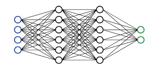
A neural network is a multi-layered model inspired by the human brain. Like the neurons in our brain, the circles represent a node. The blue circles represent the input layer, the black circles represent the hidden layers, and the green circles represent the output layer. Each node in the hidden layers represents a function that the inputs go through, ultimately leading to an output in the green circles. The formal term for these functions is called the sigmoid activation function.
6. What Is Cross-Validation?
Cross-validation is essentially a technique used to assess how well a model performs on a new, independent data set. The simplest example of cross-validation is when you split your data into two groups: training data and testing data. You use the training data to build the model and the testing data to test the model.
7. How Do You Define/Select Metrics?
There isn’t a one-size-fits-all metric. The metric(s) chosen to evaluate a machine learning model depends on various factors:
- Is it a regression or classification task?
- What is the business objective? For example, precision versus recall.
- What is the distribution of the target variable?
There are a number of metrics that can be used, including adjusted r-squared, mean absolute error (MAE), mean squared error (MSE), accuracy, recall, precision, f1 score and the list goes on.
8. Explain What Precision and Recall Are.
- Recall: Recall attempts to answer “What proportion of actual positives was identified correctly?”

- Precision: Precision attempts to answer “What proportion of positive identifications was actually correct?”

9. Explain What a False Positive and a False Negative Are. Why Is It Important to Distinguish One From the Other? Provide Examples When False Positives Are More Important Than False Negatives, False Negatives Are More Important Than False Positives and When They Are Equally Important.
- False positive: A false positive is an incorrect identification of the presence of a condition when it’s absent.
- False negative: A false negative is an incorrect identification of the absence of a condition when it’s actually present.
An example of when false negatives are more important than false positives is when screening for cancer. It’s much worse to say that someone doesn’t have cancer when they do, instead of saying that someone does and later realizing that they don’t.
This is a subjective argument, but false positives can be worse than false negatives from a psychological point of view. For example, a false positive for winning the lottery could be a worse outcome than a false negative because people normally don’t expect to win the lottery anyways.
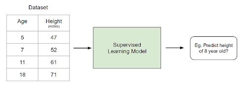
10. What Is the Difference Between Supervised Learning and Unsupervised Learning? Give Concrete Examples.
Supervised learning involves learning a function that maps an input to an output based on example input-output pairs.
For example, if I had a data set with two variables, age (input) and height (output), I could implement a supervised learning model to predict the height of a person based on their age.
Unsupervised learning is used to draw inferences and find patterns from input data without references to labeled outcomes. A common use of unsupervised learning is grouping customers by purchasing behavior to find target markets.
11. Assume You Need to Generate a Predictive Model Using Multiple Regression. Explain How You Intend to Validate This Model.
There are two main ways that you can do this: adjusted r-squared and cross-validation.
1. Adjusted R-Squared.
R-squared is a measurement that tells you to what extent the proportion of variance in the dependent variable is explained by the variance in the independent variables. In simpler terms, while the coefficients estimate trends, R-squared represents the scatter around the line of best fit.
However, every additional independent variable added to a model always increases the R-squared value. Therefore, a model with several independent variables may seem to be a better fit even if it isn’t. This is where adjusted R² comes in. The adjusted R² compensates for each additional independent variable and only increases if each given variable improves the model above what is possible by probability. This is important since we are creating a multiple regression model.
2. Cross-Validation
A method common to most people is cross-validation, splitting the data into two sets: training and testing data. Revisit the answer to the first question for more on this.
12. What Does NLP Stand For?
NLP stands for natural language processing. It’s a branch of artificial intelligence that gives machines the ability to read and understand human languages.
13. When Would You Use Random Forests vs. Support Vector Machines and Why?
There are a couple of reasons why a random forest is a better choice of model than a support vector machine (SVM):
- Random forests allow you to determine the feature importance. SVM’s can’t do this.
- Random forests are much quicker and simpler to build than an SVM.
- For multi-class classification problems, SVMs require a one-vs-rest method, which is less scalable and more memory intensive.
14. Why Is Dimension Reduction Important?
Dimensionality reduction is the process of reducing the number of features in a data set. This is important mainly in the case when you want to reduce variance in your model (overfitting).
15. What Is Principal Component Analysis? Explain the Sort of Problems You Would Use PCA for.
In its simplest sense, PCA involves projecting higher dimensional data, such as three dimensions, to a smaller space, like two dimensions. This results in a lower dimension of data, two dimensions instead of three, while keeping all original variables in the model.
PCA is commonly used for compression purposes, to reduce required memory and to speed up the algorithm, as well as for visualization purposes, making it easier to summarize data.
16. Why Is Naive Bayes Bad? How Would You Improve a Spam Detection Algorithm That Uses Naive Bayes?
One major drawback of naive Bayes is that it holds a strong assumption in that the features are assumed to be uncorrelated with one another, which typically is never the case.
One way to improve such an algorithm that uses naive Bayes is to decorrelate the features so that the assumption holds true.
17. What Are the Drawbacks of a Linear Model?
There are a couple of drawbacks to a linear model:
- A linear model holds some strong assumptions that may not be true in application. It assumes a linear relationship, multivariate normality, no or little multicollinearity, no auto-correlation and homoscedasticity
- A linear model can’t be used for discrete or binary outcomes.
- You can’t vary the model flexibility of a linear model.
18. Do You Think 50 Small Decision Trees Are Better Than a Large One? Why?
Another way of asking this question is “Is a random forest a better model than a decision tree?” And the answer is yes, because a random forest is an ensemble method that takes many weak decision trees to make a strong learner. Random forests are more accurate, more robust and less prone to overfitting.
18. Why Is Mean Square Error a Bad Measure of Model Performance? What Would You Suggest Instead?
Mean squared error (MSE) gives a relatively high weight to large errors. Therefore, MSE tends to put too much emphasis on large deviations. A more robust alternative is mean absolute deviation (MAD).
19. What Are the Assumptions Required for Linear Regression? What If Some of These Assumptions Are Violated?
The assumptions are as follows:
- The sample data used to fit the model is representative of the population.
- The relationship between X and the mean of Y is linear.
- The variance of the residual is the same for any value of X (homoscedasticity).
- Observations are independent of each other
- For any value of X, Y is normally distributed.
Extreme violations of these assumptions will make the results redundant. Small violations of these assumptions will result in a greater bias or variance of the estimate.
20. What Is Collinearity and What to Do With It? How to Remove Multicollinearity?
Multicollinearity exists when an independent variable is highly correlated with another independent variable in a multiple regression equation. This can be problematic because it undermines the statistical significance of an independent variable.
You could use the variance inflation factors (VIF) to determine if there is any multicollinearity between independent variables, a standard benchmark is that if the VIF is greater than five then multicollinearity exists.
21. How to Check If the Regression Model Fits the Data Well?
There are a couple of metrics that you can use:
- R-squared/Adjusted R-squared: Relative measure of fit.
- F1 score: Evaluates the null hypothesis that all regression coefficients are equal to zero vs the alternative hypothesis that at least one doesn’t equal zero
- Root mean-squared error (RMSE): Absolute measure of fit.
22. What Is a Decision Tree?
Decision trees are a popular model, used in operations research, strategic planning and machine learning. Each square above is called a node, and the more nodes you have, the more accurate your decision tree will be (generally). The last nodes of the decision tree, where a decision is made, are called the leaves of the tree. Decision trees are intuitive and easy to build but fall short when it comes to accuracy.
23. What Is a Random Forest? Why Is It Good?
Random forests are an ensemble learning technique that builds off of decision trees. Random forests involve creating multiple decision trees using bootstrapped data sets of the original data and randomly selecting a subset of variables at each step of the decision tree. The model then selects the mode of all of the predictions of each decision tree. By relying on a “majority wins” model, it reduces the risk of error from an individual tree.
For example, if we created one decision tree, the third one, it would predict 0. But if we relied on the mode of all four decision trees, the predicted value would be one. This is the power of random forests.
Random forests offer several other benefits including strong performance, can model non-linear boundaries, no cross-validation needed and gives feature importance.
24. What Is a Kernel? Explain the Kernel Trick.
A kernel is a way of computing the dot product of two vectors 𝐱x and 𝐲y in some, possibly very high-dimensional, feature space, which is why kernel functions are sometimes called “generalized dot product.”
The kernel trick is a method of using a linear classifier to solve a nonlinear problem by transforming linearly inseparable data to linearly separable ones in a higher dimension.
25. Is It Beneficial to Perform Dimensionality Reduction Before Fitting an SVM? Why or Why Not?
When the number of features is greater than the number of observations, then performing dimensionality reduction will generally improve the SVM.
26. What Is Overfitting?
Overfitting is an error where the model “fits” the data too well, resulting in a model with high variance and low bias. As a consequence, an overfit model will inaccurately predict new data points even though it has a high accuracy on the training data.
27. What Is Boosting?
Boosting is an ensemble method to improve a model by reducing its bias and variance, ultimately converting weak learners to strong learners. The general idea is to train a weak learner and sequentially iterate and improve the model by learning from the previous learner.
Data Science Interview Questions: Statistics, Probability and Mathematics
28. If the Probability That an Item at Location A is 0.6 and 0.8 at location B, What Is the Probability That the Item Would be Found on Amazon?
We need to make some assumptions about this question before we can answer it. Let’s assume that there are two possible places to purchase a particular item on Amazon and the probability of finding it at location A is 0.6 and B is 0.8. The probability of finding the item on Amazon can be explained as so:
We can reword the above as P(A) = 0.6 and P(B) = 0.8. Furthermore, let’s assume that these are independent events, meaning that the probability of one event is not impacted by the other. We can then use the formula:
- P(A or B) = P(A) + P(B) — P(A and B)
- P(A or B) = 0.6 + 0.8 — (0.6*0.8)
- P(A or B) = 0.92
29. You Randomly Draw a Coin From a Bag of 100 Coins. There’s One Unfair Coin (Head-Head), 99 Fair Coins (Heads-Tails). You Flip It 10 times. If the Result Is 10 Heads, What Is the Probability That the Coin Is Unfair?
This can be answered using the Bayes’ theorem. The extended equation for the Bayes theorem is the following:
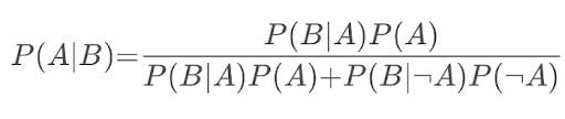
Assume that the probability of picking the unfair coin is denoted as P(A), and the probability of flipping 10 heads in a row is denoted as P(B). Then, P(B|A) is equal to 1, P(B∣¬A) is equal to 0.510, and P(¬A) is equal to 0.99.
If you fill in the equation, then P(A|B) = 0.9118 or 91.18 percent.
30. Explain the Difference Between Convex and Non-Convex Cost Function. What Does It Mean When a Cost Function Is Non-Convex?
A convex function is one where a line drawn between any two points on the graph lies on or above the graph. It has one minimum.
A non-convex function is one where a line drawn between any two points on the graph may intersect other points on the graph. It’s characterized as wavy.
When a cost function is non-convex, it means that there’s a likelihood that the function may find local minima instead of the global minimum, which is typically undesired in machine learning models from an optimization perspective.
31. Walk Through the Fundamentals of Probability
8 Rules of Probability
- For any event A, 0 ≤ P(A) ≤ 1. I other words, the probability of an event can range from zero-to-one.
- The sum of the probabilities of all possible outcomes always equals one.
- P(not A) = 1 — P(A). This rule explains the relationship between the probability of an event and its complement event. A complement event is one that includes all possible outcomes that aren’t in A.
- If A and B are disjoint events, mutually exclusive, then P(A or B) = P(A) + P(B). This is called the addition rule for disjoint events.
- P(A or B) = P(A) + P(B) — P(A and B). This is called the general addition rule.
- If A and B are two independent events, then P(A and B) = P(A) * P(B). This is called the multiplication rule for independent events.
- The conditional probability of event B given event A is P(B|A) = P(A and B) / P(A).
- For any two events A and B, P(A and B) = P(A) * P(B|A). This is called the general multiplication rule.
Counting Methods
- Factorial formula: n! = n x (n -1) x (n — 2) x … x 2 x 1. Use when the number of items is equal to the number of places available. For example, Find the total number of ways five people can sit in five empty seats. = 5 x 4 x 3 x 2 x 1 = 120.
- Fundamental counting principle: This method should be used when repetitions are allowed and the number of ways to fill an open place is not affected by previous fills. For example, there are three types of breakfasts, four types of lunches and five types of desserts. The total number of combinations is = 5 x 4 x 3 = 60.
- Permutations: P(n,r)= n! / (n−r)!. This method is used when replacements aren’t allowed and order of item ranking matters. For example, A code has 4 digits in a particular order and the digits range from 0 to 9. How many permutations are there if one digit can only be used once. P(n,r) = 10!/(10–4)! = (10x9x8x7x6x5x4x3x2x1)/(6x5x4x3x2x1) = 5040.
- Combination formula: C(n,r)=(n!)/[(n−r)!r!]. This is used when replacements are not allowed and the order in which items are ranked does not matter. For example, to win the lottery, you must select the five correct numbers in any order from one-to-52. What is the number of possible combinations? C(n,r) = 52! / (52–5)!5! = 2,598,960.
32. Describe Markov Chains.
A Markov chain is a mathematical model that predicts the probability that a sequence of events will occur based on a previous event. For example, predicting the next word to appear in a search query. It utilizes a transition matrix and initial state vector. The actual math behind Markov chains requires knowledge on linear algebra and matrices.
33. A Box has 12 Red Cards and 12 Black Cards. Another Box has 24 Red Cards and 24 Black Cards. You Want to Draw Two Cards at Random From One of the Two Boxes, One Card at a Time. Which Box has a Higher Probability of Getting Cards of the Same Color and Why?
The box with 24 red cards and 24 black cards has a higher probability of getting two cards of the same color. Let’s say the first card you draw from each deck is a red Ace.
This means that in the deck with 12 reds and 12 blacks, there’s now 11 reds and 12 blacks. Therefore your odds of drawing another red are equal to 11/(11+12) or 11/23.
In the deck with 24 reds and 24 blacks, there would then be 23 reds and 24 blacks. Therefore your odds of drawing another red are equal to 23/(23+24) or 23/47.
Since 23/47 > 11/23, the second deck with more cards has a higher probability of getting the same two cards.
34. You are at a Casino and Have Two Dice to Play With. You win $10 Every Time You Roll a 5. If You Play Until You Win and Then Stop, What Is the Expected Payout?
Let’s assume that it costs $5 every time you want to play. There are 36 possible combinations with two dice.
Of the 36 combinations, there are four combinations that result in rolling a five. This means that there is a 4/36 or 1/9 chance of rolling a five. A 1/9 chance of winning means you’ll lose eight times and win once (theoretically).
Therefore, your expected payout is equal to $10.00 * 1 — $5.00 * 9= -$35.00.
35. How Can You Tell If a Given Coin Is Biased?
This isn’t a trick question. The answer is simply to perform a hypothesis test:
- The null hypothesis is that the coin is not biased and the probability of flipping heads should equal 50 percent (p=0.5). The alternative hypothesis is that the coin is biased and p != 0.5.
- Flip the coin 500 times.
- Calculate the Z-score. If the sample is less than 30, you would calculate the t-statistics.
- Compare against the alpha, Two-tailed test, so 0.05/2 = 0.025.
- If p-value > alpha, the null is not rejected and the coin is not biased. If p-value < alpha, the null is rejected and the coin is biased.
36. Make an Unfair Coin Fair.
Since a coin flip is a binary outcome, you can make an unfair coin fair by flipping it twice. If you flip it twice, there are two outcomes that you can bet on: heads followed by tails or tails followed by heads.
P(heads) * P(tails) = P(tails) * P(heads)
This makes sense since each coin toss is an independent event. This means that if you get heads → heads or tails → tails, you would need to reflip the coin.
37. You Are About to Get on a Plane to London, and You Want to Know Whether You Have to Bring an Umbrella or Not. You Call Three of Your Random Friends and Ask Each One of them If It’s Raining. The Probability That Your Friend Is Telling the Truth Is ⅔, and the Probability That They’re Playing a Prank on You by Lying is 1/3. If all 3 of Them Say That It’s Raining, What Is the Probability That It’s Actually Raining in London?
You can tell that this question is related to Bayes' theorem because of the last statement, which essentially follows the structure, “What is the probability A is true given B is true?” Therefore we need to know the probability of it raining in London on a given day. Let’s assume it’s 25 percent.
- P(A) is the probability of it raining, which equals 25 percent
- P(B) is the probability of all three friends say that it’s raining.
- P(A|B) is the probability that it’s raining given they say that it’s raining.
- P(B|A) probability that all three friends say that it’s raining given it’s raining = (2/3)³ = 8/27.
Step 1: Solve for P(B)
- P(A|B) = P(B|A) * P(A) / P(B), can be rewritten as P(B) = P(B|A) * P(A) + P(B|not A) * P(not A).
- P(B) = (2/3)³ * 0.25 + (1/3)³ * 0.75 = 0.25*8/27 + 0.75*1/27
Step 2: Solve for P(A|B)
- P(A|B) = 0.25 * (8/27) / ( 0.25*8/27 + 0.75*1/27)
- P(A|B) = 8 / (8 + 3) = 8/11
Therefore, if all three friends say that it’s raining, then there’s an 8/11 chance that it’s actually raining.
38. You’re given 40 Cards With Four Different Colors — 10 Green Cards, 10 Red Cards, 10 Blue Cards and 10 Yellow Cards. The Cards of Each Color Are Numbered From One to 10. Two Cards Are Picked at Random. Find Out the Probability That the Cards Picked Aren’t the Same Number and Same Color.
Since these events aren’t independent, we can use the rule:
P(A and B) = P(A) * P(B|A), which is also equal to P(not A and not B) = P(not A) * P(not B | not A).
For example:
- P(not 4 and not yellow) = P(not 4) * P(not yellow | not 4)
- P(not 4 and not yellow) = (36/39) * (27/36)
- P(not 4 and not yellow) = 0.692
Therefore, the probability that the cards picked are not the same number and the same color is 69.2 percent.
39. How Do You Assess the Statistical Significance of an Insight?
You would perform hypothesis testing to determine statistical significance. First, you would state the null hypothesis and alternative hypothesis. Second, you would calculate the p-value, the probability of obtaining the observed results of a test assuming that the null hypothesis is true. Last, you would set the level of the significance (alpha), and if the p-value is less than the alpha, you would reject the null. In other words, the result is statistically significant.
40. Explain What a Long-Tailed Distribution Is and Provide Three Examples of Relevant Phenomena That Have Long Tails. Why Are They Important in Classification and Regression Problems?
A long-tailed distribution is a type of heavy-tailed distribution that has a tail (or tails) that drops off gradually and asymptotically.
Three practical examples include the power law, the Pareto principle, more commonly known as the 80–20 rule and product sales (i.e., best selling products versus others).
It’s important to be mindful of long-tailed distributions in classification and regression problems because the least frequently occurring values make up the majority of the population. This can ultimately change the way that you deal with outliers, and it also conflicts with some machine learning techniques with the assumption that the data is normally distributed.
41. What Is the Central Limit Theorem? Why Is It Important?
Central limit theorem is the statistical concept that as a sample size expands, the mean of all samples will equal the mean of the population, and the distribution of means will follow a normal distribution.
The central limit theorem is important because it is used in hypothesis testing and also to calculate confidence intervals.
43. What Is Statistical Power?
‘Statistical power’ refers to the power of a binary hypothesis, which is the probability that the test rejects the null hypothesis given that the alternative hypothesis is true.

44. Explain Selection Bias With Regard to a Data Set, Not Variable Selection. Why Is It Important? How Can Data Management Procedures, Such as Missing Data Handling, Make It Worse?
Selection bias is the phenomenon of selecting individuals, groups or data for analysis in such a way that proper randomization is not achieved, ultimately resulting in a sample that is not representative of the population.
Understanding and identifying selection bias is important because it can significantly skew results and provide false insights about a particular population group.
Types of selection bias include:
- Sampling bias: A biased sample caused by non-random sampling.
- Time interval: Selecting a specific time frame that supports the desired conclusion. For example, conducting a sales analysis near Christmas.
- Exposure: This includes clinical susceptibility bias, protopathic bias, indication bias.
- Data: Includes cherry-picking, suppressing evidence and the fallacy of incomplete evidence.
- Attrition: Attrition bias is similar to survivorship bias, where only those that ‘survived’ a long process are included in an analysis, or failure bias, where those that failed are only included
- Observer selection: Related to the Anthropic principle, which is a philosophical consideration that any data we collect about the universe is filtered by the fact that, in order for it to be observable, it must be compatible with the conscious and sapient life that observes it.
Handling missing data can make selection bias worse because different methods impact the data in different ways. For example, if you replace null values with the mean of the data, you’re adding bias in the sense that you’re assuming that the data is not as spread out as it might actually be.
45. Provide a Simple Example of How an Experimental Design Can Help Answer a Question About Behavior. How Does Experimental Data Contrast With Observational Data?
Observational data comes from observational studies, which are when you observe certain variables and try to determine if there is any correlation.
Experimental data comes from experimental studies, which are when you control certain variables and hold them constant to determine if there is any causality.
An example of experimental design is the following: split a group up into two. The control group lives their lives normally. The test group is told to drink a glass of wine every night for 30 days. Then research can be conducted to see how wine affects sleep.
46. Is Mean Imputation of Missing Data Acceptable Practice? Why or Why Not?
Mean imputation is the practice of replacing null values in a data set with the mean of the data.
Mean imputation is generally bad practice because it doesn’t take into account feature correlation. For example, imagine we have a table showing age and fitness score and imagine that an 80-year-old has a missing fitness score. If we took the average fitness score from an age range of 15-to-80 years old, then the 80-year-old will appear to have a much higher fitness score than they actually should.
Second, mean imputation reduces the variance of the data and increases bias in our data. This leads to a less accurate model and a narrower confidence interval due to a smaller variance.
47. What Is an Outlier? Explain How You’d Screen for Outliers and What You’d Do If You Found Them in Your Data Set. Explain What an Inlier Is, How You’d Screen for Them and What You’d Do If You Found Them in Your Data Set.
An outlier is a data point that differs significantly from other observations.
Depending on the cause of the outlier, they can be bad from a machine learning perspective because they can worsen the accuracy of a model. If a measurement error caused the outlier, it’s important to remove them from the data set. There are a couple of ways to identify outliers.
Z-Score/Standard Deviations
If we know that 99.7 percent of data in a data set lies within three standard deviations, then we can calculate the size of one standard deviation, multiply it by 3, and identify the data points that are outside of this range. Likewise, we can calculate the z-score of a given point, and if it’s equal to plus-or-minus three, then it’s an outlier. There are a few contingencies that need to be considered when using this method. The data must be normally distributed, this is not applicable for small data sets, and the presence of too many outliers can throw off z-score.
Interquartile Range (IQR)
IQR, the concept used to build boxplots, can also be used to identify outliers. The IQR is equal to the difference between the third quartile and the first quartile. You can then identify if a point is an outlier if it is less than Q1–1.5*IRQ or greater than Q3 + 1.5*IQR. This comes to approximately 2.698 standard deviations.
Other methods include DBScan clustering, isolation forests and robust random cut forests.
Inlier
An inlier is a data observation that lies within the rest of the data set and is unusual or an error. Since it lies in the data set, it is typically harder to identify than an outlier and requires external data to identify them. Should you identify any inliers, you can simply remove them from the data set to address them.
48. How Do You Handle Missing Data? What Imputation Techniques Do You Recommend?
There are several ways to handle missing data:
- Delete rows with missing data.
- Mean/Median/Mode imputation.
- Assigning a unique value.
- Predicting the missing values.
- Using an algorithm which supports missing values, like random forests.
The best method is to delete rows with missing data as it ensures that no bias or variance is added or removed, and ultimately results in a robust and accurate model. However, this is only recommended if there’s a lot of data to start with and the percentage of missing values is low.
49. You Have Data on the Duration of Calls to a Call Center. Generate a Plan for How You Would Code and Analyze the Data. Explain a Plausible Scenario for What the Distribution of These Durations Might Look Like. How Could You Test, Even Graphically, Whether Your Expectations Are Accurate?
First I would conduct an exploratory data analysis (EDA) to clean, explore, and understand my data. As part of my EDA, I could compose a histogram of the duration of calls to see the underlying distribution.
My guess is that the duration of calls would follow a lognormal distribution. The reason that I believe it’s positively skewed is because the lower end is limited to zero, since a call can’t be negative seconds. However, on the upper end, it’s likely for there to be a small proportion of calls that are extremely long relatively.
You could use a Q-Q plot to confirm whether the duration of calls follows a lognormal distribution or not.
50. Explain Likely Differences Between Administrative Data Sets and Data Sets Gathered From Experimental Studies. What Are Likely Problems Encountered With Administrative Data? How Do Experimental Methods Help Alleviate These Problems? What Problem Do They Bring?
Administrative data sets are typically data sets used by governments or other organizations for non-statistical reasons.
Administrative data sets are usually larger and more cost-efficient than experimental studies. They are also regularly updated assuming that the organization associated with the administrative data set is active and functioning. At the same time, administrative data sets may not capture all of the data that one may want and may not be in the desired format either. It is also prone to quality issues and missing entries.
51. You Are Compiling a Report for User Content Uploaded Every Month and Notice a Spike in Picture Uploads in October. What Might You Think Is the Cause of This, and How Would You Test It?
There are a number of potential reasons for a spike in photo uploads:
- A new feature may have been implemented in October which involves uploading photos and gained a lot of traction by users. For example, a feature that gives the ability to create photo albums.
- Similarly, it’s possible that the process of uploading photos before was not intuitive and was improved in the month of October.
- There may have been a viral social media movement that involved uploading photos that lasted for all of October. For example, Movember but something more scalable.
- It’s possible that the spike is due to people posting pictures of themselves in costumes for Halloween.
The method of testing depends on the cause of the spike, but you would conduct hypothesis testing to determine if the inferred cause is the actual cause.
52. Give Examples of Data That Doesn’t Have a Gaussian Distribution, Nor Log-Normal
- Any type of categorical data won’t have a gaussian distribution or lognormal distribution.
- Exponential distributions: For example, the amount of time that a car battery lasts or the amount of time until an earthquake occurs.
53. What Is Root Cause Analysis? How to Identify a Cause vs. a Correlation? Give Examples
Root cause analysis is a method of problem-solving used for identifying the root cause(s) of a problem.
Correlation measures the relationship between two variables, ranging from -1 to 1. Causation is when a first event appears to have caused a second event. Causation essentially looks at direct relationships while correlation can look at both direct and indirect relationships.
For example, a higher crime rate is associated with higher sales in ice cream in Canada, in other words, they are positively correlated. However, this doesn’t mean that one causes another. Instead, it’s because both occur more when it’s warmer outside.
You can test for causation using hypothesis testing or A/B testing.
54. Give an example where the median is a better measure than the mean
When there are a number of outliers that positively or negatively skew the data.
55. Given Two Fair Dice, What Is the Probability of Getting Scores That Sum to Four? To Eight?
There are four combinations of rolling a four (1+3, 3+1, 2+2):
- P(rolling a 4) = 3/36 = 1/12.
There are combinations of rolling an eight (2+6, 6+2, 3+5, 5+3, 4+4):
- P(rolling an 8) = 5/36.
56. What Is the Law of Large Numbers?
The law of large numbers is a theory that states that as the number of trials increases, the average of the result will become closer to the expected value.
For example, flipping heads using a fair coin 100,000 times should be closer to 0.5 than 100 times.
57. How Do You Calculate the Needed Sample Size?

You can use the margin of error (ME) formula to determine the desired sample size.
- t/z: t/z score used to calculate the confidence interval
- M: the desired margin of error
- S: sample standard deviation
58. When You Sample, What Bias Are You Inflicting?
Potential biases include the following:
- Sampling bias: A biased sample caused by non-random sampling.
- Under coverage bias: Sampling too few observations.
- Survivorship bias: Error of overlooking observations that did not make it past a form of selection process.
59. How Do You Control for Biases?
There are many things that you can do to control and minimize bias. Two common things include randomization, where participants are assigned by chance, and random sampling, sampling in which each member has an equal probability of being chosen.
60. What Are Confounding Variables?
A confounding variable, or a confounder, is a variable that influences both the dependent variable and the independent variable, causing a spurious association, a mathematical relationship in which two or more variables are associated but not causally related.
61. What Is A/B Testing?
A/B testing is a form of hypothesis testing and two-sample hypothesis testing to compare two versions, the control and variant, of a single variable. It is commonly used to improve and optimize user experience and marketing.
62. How Do You Prove That Males Are on Average Taller Than Females?
You can use hypothesis testing to prove that males are taller on average than females.
The null hypothesis would state that males and females are the same height on average, while the alternative hypothesis would state that the average height of males is greater than the average height of females.
Then you would collect a random sample of heights of males and females and use a t-test to determine if you reject the null or not.
63. Infection Rates at a Hospital Above a 1 Infection per 100 Person-Days at Risk Are Considered High. Suppose a Hospital Had 10 Infections over the last 1787 person-days at risk. Give the P-Value of the Correct One-Sided Test of Whether the Hospital Is Below the Standard.
Since we’re looking at the number of events (# of infections) occurring within a given timeframe, this is a Poisson distribution question.
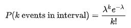
- Null (H0) = 1 infection per person-days
- Alternative (H1) = greater than 1 infection per person-days
- k (actual) = 10 infections
- lambda (theoretical) = (1/100)*1787
- p = 0.032372 or 3.2372 percent. Answer calculated using
.poisson()in Excel orppoisin R.
Since p-value < alpha (assuming 5 percent level of significance), we reject the null and conclude that the hospital is below the standard.
64. You Flip a Biased Coin (p(head)=0.8) Five Times. What’s the Probability of Getting Heads Three or More Times?
Use the general binomial probability formula to answer this question:

- p = 0.8
- n = 5
- k = 3,4,5
- P(3 or more heads) = P(3 heads) + P(4 heads) + P(5 heads) = 0.94 or 94 percent.
65. A Random Variable X Is Normal With Mean 1020 and a Standard Deviation 50. Calculate P(X>1200).
Using Excel:
p = 1-norm.dist(1200, 1020, 50, true)p = 0.000159
66. Consider the Number of People Who Show Up at a Bus Station Is Poisson with Mean 2.5/h. What Is the Probability That at Most Three People Show Up in a Four Hour Period?
- x = 3
- mean = 2.5*4 = 10
Using Excel to solve:
p = poisson.dist(3,10,true)p = 0.010336
67. An HIV Test Has a Sensitivity of 99.7 Percent and a Specificity of 98.5 Percent. A Subject From a Population of Prevalence 0.1 Percent Receives a Positive Test Result. What Is the Precision of the Test, i.e. the Probability They Are HIV Positive?
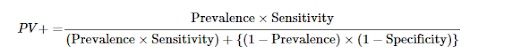
- Precision: Positive predictive value, which equals PV
- PV = (0.001*0.997)/[(0.001*0.997)+((1–0.001)*(1–0.985))]
- PV = 0.0624 or 6.24 percent
68. You Are Running for Office and Your Pollster Polled 100 People. Sixty of Them Claimed They’ll Vote for You. Can You Relax?
First we need to make a few assumptions:
- Assume that there’s only you and one other opponent.
- Also, assume that we want a 95 percent confidence interval. This gives us a z-score of 1.96.
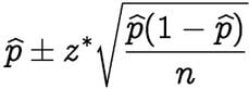
- p-hat = 60/100 = 0.6
- z* = 1.96
- n = 100
This gives us a confidence interval of [50.4,69.6]. Therefore, given a confidence interval of 95 percent. If you are okay with the worst scenario of tying, then you can relax. Otherwise, you can’t relax until you receive 61 out of 100 to claim yes.
69. A Geiger Counter Records 100 Radioactive Decays in 5 Minutes. Find an Approximate 95 Percent Interval for the Number of Decays Per Hour.
- Since this is a Poisson distribution question, mean = lambda = variance, which also means that standard deviation = square root of the mean.
- A 95 percent confidence interval implies a z score of 1.96.
- One standard deviation = 10.
Therefore, the confidence interval = 100 +/- 19.6 = [964.8, 1435.2].
70. The Homicide Rate in Scotland Fell Last Year to 99 From 115 the year before. Is This Reported Change Noteworthy?
- Since this is a Poisson distribution question, mean = lambda = variance, which also means that standard deviation = square root of the mean
- A 95 percent confidence interval implies a z score of 1.96.
- One standard deviation = sqrt(115) = 10.724
Therefore the confidence interval = 115+/- 21.45 = [93.55, 136.45]. Since 99 is within this confidence interval, we can assume that this change is not very noteworthy.
71. Consider the Influenza Epidemic for Two-Parent Heterosexual Families. Suppose There’s a 17 Percent Probability That at Least One of the Parents Has Contracted the Disease. There’s a 12 Percent Probability That the Father Has Contracted Influenza and a 6 Percent Probability That Both the Mother and Father Have Contracted the Disease. What Is the Probability That the Mother HasContracted Influenza?
Using the general addition rule in probability:
- P(mother or father) = P(mother) + P(father) — P(mother and father)
- P(mother) = P(mother or father) + P(mother and father) — P(father)
- P(mother) = 0.17 + 0.06–0.12
- P(mother) = 0.11
72. Suppose That Diastolic Blood Pressures (DBPs) for Men Aged 35-to-44 Years Old Are Normally Distributed With a Mean of 80 mm Hg and a Standard Deviation of 10. What’s the Probability That a Random 35-to-44 Year Old has a DBP Less Than 70?
Since 70 is one standard deviation below the mean, take the area of the Gaussian distribution to the left of one standard deviation, which equals 2.3 + 13.6 = 15.9 percent
73. In a Population of Interest, a Sample of 9 Men Yielded a Sample Average Brain Volume of 1,100cc and a Standard Deviation of 30cc. What Is a 95 Percent Student’s T-Confidence Interval for the Mean Brain Volume in This New Population?

Given a confidence level of 95 percent and degrees of freedom equal to 8, the t-score = 2.306.
- Confidence interval = 1100 +/- 2.306*(30/3)
- Confidence interval = [1076.94, 1123.06]
74. A Diet Pill Is Given to 9 Subjects Over Six Weeks. The Average Difference in Weight (Follow Up — Baseline) Is -2 Pounds. What Would the Standard Deviation of the Difference in Weight Have to Be for the Upper Endpoint of the 95 Percent T-Confidence Interval to Touch 0?
- Upper bound = mean + t-score*(standard deviation/sqrt(sample size))
- 0 = -2 + 2.306*(s/3)
- 2 = 2.306 * s / 3
- s = 2.601903
Therefore, the standard deviation would have to be at least approximately 2.60 for the upper bound of the 95 percent T-confidence interval to touch 0.
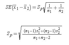
75. In a Study of Emergency Room Wait Times, Investigators Compare a New Triage System to the Standard. To Test the Systems, Administrators Selected 20 Nights and Randomly Assigned the New System to Be Used on 10 nights and the Standard System on the Remaining 10 Nights. They Calculated the Nightly Median Waiting Time (MWT) to See a Physician. The Average MWT for the New System Was 3 Hours With a Variance of 0.60, While the Average MWT for the Old System Was 5 Hours With a Variance of 0.68. Consider the 95 Percent Confidence Interval Estimate for the Differences of the Mean MWT Associated With the New System. Assume a Constant Variance. What Is the Interval? Subtract in this order (New System — Old System).
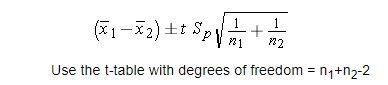
- Confidence Interval = mean +/- t-score * standard error.
- mean = new mean — old mean = 3–5 = -2
- T-score = 2.101 given df=18 (20–2) and confidence interval of 95 percent.

- Standard error = sqrt((0.⁶²*9+0.⁶⁸²*9)/(10+10–2)) * sqrt(1/10+1/10)
- Standard error = 0.352
- Confidence interval = [-2.75, -1.25]
76. To Further Test the Hospital Triage System, Administrators Selected 200 Nights and Randomly Assigned a New Triage System to Be Used on 100 Nights, and a Standard System on the Remaining 100 Nights. They Calculated the Nightly Median Waiting Time (MWT) to See a Physician. The Average MWT for the New System Was 4 Hours With a Standard Deviation of 0.5 hours, While the Average MWT for the Old System Was 6 Hours With a Standard Deviation of 2 Hours. Consider the Hypothesis of a Decrease in the Mean MWT Associated With the New Treatment. What Does the 95 Percent Independent Group Confidence Interval With Unequal Variances Suggest With This Hypothesis? Use the Z Quantile Instead of the T.
Assuming we subtract in this order (New System — Old System):
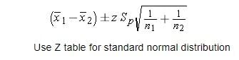
- Confidence interval formula for two independent samples
- Mean = new mean — old mean = 4–6 = -2.
- Z-score = 1.96 confidence interval of 95 percent.
- St. error = sqrt((0.⁵²*99+²²*99)/(100+100–2)) * sqrt(1/100+1/100)
- Standard error = 0.205061
- Lower bound = -2–1.96*0.205061 = -2.40192
- Upper bound = -2+1.96*0.205061 = -1.59808
- Confidence interval = [-2.40192, -1.59808]
Data Science Interview: SQL Practice Problems
77. Second Highest Salary
Write a SQL query to get the second highest salary from the Employee table. For example, given the Employee table below, the query should return 200 as the second highest salary. If there is no second highest salary, then the query should return null.
+----+--------+
| Id | Salary |
+----+--------+
| 1  | 100    |
| 2  | 200    |
| 3  | 300    |
+----+--------+
Solution A: Using IFNULL, OFFSET
IFNULL(expression, alt) :Ifnull()returns the specified value ifnull, otherwise it returns the expected value. We’ll use this to return null if there’s no second-highest salary.OFFSET: Offset is used with theORDER BYclause to disregard the top n rows that you specify. This will be useful as you’ll want to get the second row (second highest salary).
SELECT
    IFNULL(
        (SELECT DISTINCT Salary
        FROM Employee
        ORDER BY Salary DESC
        LIMIT 1 OFFSET 1
        ), null) as SecondHighestSalary
FROM Employee
LIMIT 1
SOLUTION B: Using MAX()
This query says to choose the MAX salary that isn’t equal to the MAX salary, which is equivalent to saying to choose the second-highest salary.
SELECT MAX(salary) AS SecondHighestSalary
FROM Employee
WHERE salary != (SELECT MAX(salary) FROM Employee)
78. Duplicate Emails
Write a SQL query to find all duplicate emails in a table named Person.
+----+---------+
| Id | Email   |
+----+---------+
| 1  | [email protected] |
| 2  | [email protected] |
| 3  | [email protected] |
+----+---------+
Solution A: COUNT() in a Subquery
First, a subquery is created to show the count of the frequency of each email. Then, the subquery is filtered WHERE the count is greater than 1.
SELECT Email
FROM (
    SELECT Email, count(Email) AS count
    FROM Person
    GROUP BY Email
) as email_count
WHERE count > 1
Solution B: HAVING Clause
HAVING is a clause that essentially allows you to use a WHERE statement in conjunction with aggregates (GROUP BY).
SELECT Email
FROM Person
GROUP BY Email
HAVING count(Email) > 1
79. Rising Temperature
Given a Weather table, write an SQL query to find all dates’ Ids with higher temperature compared to its previous (yesterday’s) dates.
+---------+------------------+------------------+
| Id(INT) | RecordDate(DATE) | Temperature(INT) |
+---------+------------------+------------------+
|       1 |       2015-01-01 |               10 |
|       2 |       2015-01-02 |               25 |
|       3 |       2015-01-03 |               20 |
|       4 |       2015-01-04 |               30 |
+---------+------------------+------------------+
Solution: DATEDIFF()
DATEDIFF calculates the difference between two dates and is used to make sure we’re comparing today’s temperature to yesterday’s temperature. In plain words, the query is saying, “Select the Ids where the temperature on a given day is greater than the temperature yesterday.”
SELECT DISTINCT a.Id
FROM Weather a, Weather b
WHERE a.Temperature > b.Temperature
AND DATEDIFF(a.Recorddate, b.Recorddate) = 1
80. Department Highest Salary
The Employee table holds all employees. Every employee has an Id, a salary, and there is also a column for the departmentId.
+----+-------+--------+--------------+
| Id | Name  | Salary | DepartmentId |
+----+-------+--------+--------------+
| 1  | Joe   | 70000  | 1            |
| 2  | Jim   | 90000  | 1            |
| 3  | Henry | 80000  | 2            |
| 4  | Sam   | 60000  | 2            |
| 5  | Max   | 90000  | 1            |
+----+-------+--------+--------------+
The Department table holds all departments of the company.
+----+----------+
| Id | Name     |
+----+----------+
| 1  | IT       |
| 2  | Sales    |
+----+----------+
Write an SQL query to find employees who have the highest salary in each of the departments. For the above tables, your SQL query should return the following rows (order of rows does not matter).
+------------+----------+--------+
| Department | Employee | Salary |
+------------+----------+--------+
| IT         | Max      | 90000  |
| IT         | Jim      | 90000  |
| Sales      | Henry    | 80000  |
+------------+----------+--------+
Solution: IN Clause
- The
INclause allows you to use multipleORclauses in aWHEREstatement. For example,WHERE country = ‘Canada’orcountry = ‘USA’is the same asWHERE country IN (‘Canada’, ’USA’). - In this case, we want to filter the
Departmenttable to only show the highestSalaryper Department (i.e.DepartmentId). Then we can join the two tablesWHEREtheDepartmentIdandSalaryis in the filteredDepartmenttable.
SELECT
    Department.name AS 'Department',
    Employee.name AS 'Employee',
    Salary
FROM Employee
INNER JOIN Department ON Employee.DepartmentId = Department.Id
WHERE (DepartmentId , Salary)
    IN
    (   SELECT
            DepartmentId, MAX(Salary)
        FROM
            Employee
        GROUP BY DepartmentId
 )
81: Exchange Seats
Mary is a teacher in a middle school and she has a table seat storing students’ names and their corresponding seat ids. The column id is a continuous increment. Mary wants to change seats for the adjacent students.
Can you write a SQL query to output the result for Mary?
+---------+---------+
|    id   | student |
+---------+---------+
|    1    | Abbot   |
|    2    | Doris   |
|    3    | Emerson |
|    4    | Green   |
|    5    | Jeames  |
+---------+---------+
For the sample input, the output is:
+---------+---------+
|    id   | student |
+---------+---------+
|    1    | Doris   |
|    2    | Abbot   |
|    3    | Green   |
|    4    | Emerson |
|    5    | Jeames  |
+---------+---------+
If the number of students is odd, there is no need to change the last one’s seat.
Solution: CASE WHEN
- Think of a
CASE WHEN THENstatement like anIFstatement in coding. - The first
WHENstatement checks to see if there’s an odd number of rows, and if there is, ensures that the id number does not change. - The second
WHENstatement adds 1 to each id. For example, 1,3,5 becomes 2,4,6. - Similarly, the third
WHENstatement subtracts 1 to each id. For example, 2,4,6 becomes 1,3,5.
SELECT
    CASE
        WHEN((SELECT MAX(id) FROM seat)%2 = 1) AND id = (SELECT MAX(id) FROM seat) THEN id
        WHEN id%2 = 1 THEN id + 1
        ELSE id - 1
    END AS id, student
FROM seat
ORDER BY id
Data Science Interview Questions Miscellaneous
82. If There Are 8 Marbles of Equal Weight and 1 Marble That Weighs a Little More For a Total of 9 Marbles, How Many Weighings Are Required to Determine Which Marble Is Heaviest?
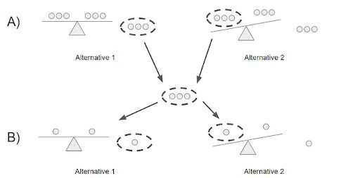
Two weighings would be required (see part A and B above):
- You would split the nine marbles into three groups of three and weigh two of the groups. If the scale balances (alternative 1), you know that the heavy marble is in the third group of marbles. Otherwise, you’ll take the group that weighed more heavily (alternative 2).
- Then, you would exercise the same step, but you’d have three groups of one marble instead of three groups of three.
83. How Would a Change of Amazon Prime’s Membership Fee Affect the Market?
Let’s take the instance where there’s an increase in the prime membership fee. There are two parties involved, the buyers and the sellers.
For the buyers, the impact of an increase in a Prime membership fee ultimately depends on the price elasticity of demand for the buyers. If the price elasticity is high, then a given price increase will result in a large drop in demand and vice versa. Buyers that continue to purchase a membership fee are likely Amazon’s most loyal and active customers. They’re also likely to place a higher emphasis on products with Prime.
Sellers will take a hit, as there is now a higher cost of purchasing Amazon’s basket of products. That being said, some products will take a harder hit while others may not be impacted. It’s likely that premium products that Amazon’s most loyal customers purchase would not be affected as much, like electronics.
84. If 70 Percent of Facebook Users on iOS Use Instagram, But Only 35 Percent of Users on Android Use Instagram, How Would You Investigate the Discrepancy?
There are a number of possible variables that can cause such a discrepancy that I would check to see:
- The demographics of iOS and Android users might differ significantly. For example, according to Hootsuite, 43 percent of females use Instagram as opposed to 31 percent of men. If the proportion of female users for iOS is significantly larger than for Android, then this can explain the discrepancy, or at least a part of it. This can also be said for age, race, ethnicity and location, etc.
- Behavioral factors can also have an impact on the discrepancy. If iOS users use their phones more heavily than Android users, it’s more likely that they’ll indulge in Instagram and other apps than someone who spent significantly less time on their phones.
- Another possible factor to consider is how Google Play and the App Store differ. For example, if Android users have significantly more apps (and social media apps) to choose from, that may cause greater dilution of users.
- Lastly, any differences in the user experience can deter Android users from using Instagram compared to iOS users. If the app is more buggy for Android users than iOS users, they’ll be less likely to be active on the app.
85. Likes Per User and Minutes Spent on a Platform Are Increasing but Total Number of Users Are Decreasing. What Could Be the Root Cause of It?
Generally, you would want to probe the interviewer for more information but let’s assume that this is the only information that they are willing to give.
Focusing on likes per user, there are two reasons why this would have gone up. The first reason is that the engagement of users has generally increased on average over time — this makes sense because as time passes, active users are more likely to be loyal users as using the platform becomes a habitual practice. The other reason why likes per user would increase is that the denominator, the total number of users, is decreasing. Assuming that users that stop using the platform are inactive users, or users with little engagement and fewer likes than average, this would increase the average number of likes per user.
The explanation above can also be applied to minutes spent on the platform. Active users are becoming more engaged over time, while users with little usage are becoming inactive. Overall the increase in engagement outweighs the users with little engagement.
To take it a step further, it’s possible that the ‘users with little engagement’ are bots that Facebook has been able to detect. But over time, Facebook has been able to develop algorithms to spot and remove bots. If there were a significant number of bots before, this can potentially be the root cause of this phenomenon.
86. Facebook Likes Are Up 10 Percent Year-Over-Year. Why Could This Be?
The total number of likes in a given year is a function of the total number of users and the average number of likes per user, which I’ll refer to as engagement.
Some potential reasons for an increase in the total number of users are the following: Uusers acquired due to international expansion and younger age groups signing up for Facebook as they get older.
Some potential reasons for an increase in engagement are an increase in usage of the app from users that are becoming more and more loyal, new features and functionality and an improved user experience.
87. If We Were Testing Product X, What Metrics Would You Look at to Determine If It’s a Success?
The metrics that determine a product’s success are dependent on the business model and what the business is trying to achieve through the product. The book Lean Analytics: Use Data to Build a Better Startup Faster lays out a great framework that one can use to determine what metrics to use in a given scenario.
88. If a PM Says That They Want to Double the Number of Ads in NewsFeed, How Would You Figure Out If This Is a Good Idea or Not?
You can perform an A/B test splitting the users into two groups: a control group with the normal number of ads and a test group with double the number of ads. Then you would choose the metric to define what a “good idea” is. For example, we can say that the null hypothesis is that doubling the number of ads will reduce the time spent on Facebook and the alternative hypothesis is that doubling the number of ads won’t have any impact on the time spent on Facebook. However, you can choose a different metric like the number of active users or the churn rate. Then you would conduct the test and determine the statistical significance of the test to reject or not reject the null.
89. Define Lift, KPI, Robustness, Model Fitting, Design of Experiments and the 80/20 Rule?
Lift
lift is a measure of the performance of a targeting model measured against a random choice targeting model. In other words, lift tells you how much better your model is at predicting things than if you had no model.
KPI
KPI stands for key performance indicator, which is a measurable metric used to determine how well a company is achieving its business objectives. For example, error rate.
Robustness
Generally, robustness refers to a system’s ability to handle variability and remain effective.
Model Fitting
Model fitting refers to how well a model fits a set of observations.
Design of Experiments
Also known as DOE, design of experiments is the design of any task that aims to describe and explain the variation of information under conditions that are hypothesized to reflect the variable. In essence, an experiment aims to predict an outcome based on a change in one or more inputs (independent variables.
80/20 Rule
Also known as the Pareto principle, the 80/20 rule states that 80 percent of the effects come from 20 percent of the causes. For example, 80 percent of sales come from 20 percent of the customers.
90. Define Quality Assurance and Six Sigma.
- Quality assurance: An activity or set of activities focused on maintaining a desired level of quality by minimizing mistakes and defects.
- Six sigma: Six sigma is a specific type of quality assurance methodology composed of a set of techniques and tools for process improvement. A six sigma process is one in which 99.99966 percent of all outcomes are free of defects.
Frequently Asked Questions
What topics are commonly covered in data science interviews?
Data science interviews often cover machine learning, probability, statistics, SQL, experimental design and business problem-solving.
How should I prepare for machine learning questions in an interview?
Understand key concepts like overfitting, regularization (L1 and L2), supervised vs. unsupervised learning, neural networks and model evaluation metrics such as precision and recall.
What SQL problems should I expect in a data science interview?
Expect queries that test your ability to use GROUP BY, JOIN, HAVING, MAX() and subqueries. Common tasks include finding the second-highest salary, detecting duplicates, and analyzing trends.
How are probability and statistics tested in interviews?
Interviewers may ask about Bayes’ theorem, conditional probability, Poisson distributions, the central limit theorem, and statistical significance, often through real-world scenarios.


