Demystifying R-Squared and Adjusted R-Squared

R-squared (or the coefficient of determination) measures the variation that is explained by a regression model. For a multiple regression model, R-squared increases or remains the same as we add new predictors to the model, even if the newly added predictors are independent of the target variable and don’t add any value to the predicting power of the model. Adjusted R-squared eliminates this drawback. It only increases if the newly added predictor improves the model’s predicting power.

In this article, we’ll discuss the math behind R-squared and adjusted R-squared along with a few important concepts like explained variation, unexplained variation and total variation. We’ll implement R-squared and adjusted R-squared in Python. We’ll also see why adjusted R-squared is a reliable measure of goodness of fit for multiple regression problems.

R-Squared Terms to Know

Before proceeding with R-squared, it’s essential to understand a few terms like total variation, explained variation and unexplained variation. Imagine a world without predictive modeling, where we are tasked with predicting the price of a house given the prices of other houses. In such cases, we’d have no other option but to choose the most common value — the mean of the other house prices — as our prediction. For example, if the mean price for 100 houses is $100,000, and we were asked to predict the price of a new house, our prediction would be $100,000. That’s because we have no other data to help with our prediction.

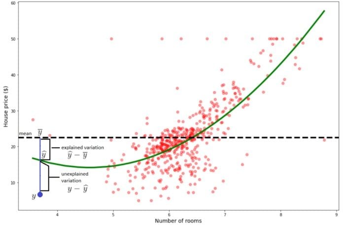
The plot shows house prices versus the number of rooms. The black dashed line is the mean of the already available house prices (target variable of the training set). The green line is the regression model of the house price with number of rooms as the predictor. The blue dot is the number of rooms for which we have to predict the house price. The true/actual house price (y) of the blue dot is five. The predicted value (y-hat) is 16. The mean value (y-bar) of the already available house prices is 21.

If we had to predict the house price of the blue dot without using the number of rooms predictor, then our prediction would be y-bar, i.e. 21. If we use a regression model with the number of rooms as a predictor, then our prediction would be y-hat, i.e. 16.

More on Data Science: Using T-SNE in Python to Visualize High-Dimensional Data Sets

Explained Variation

Explained variation is the difference between the predicted value (y-hat) and the mean of already available ‘y’ values (y-bar). It is the variation in ‘y’ that is explained by a regression model.

Unexplained Variation

Unexplained variation is the difference between true/actual value (y) and y-hat. It’s the variation in ‘y’ that is not captured/explained by a regression model. It’s also known as the residual of a regression model.

Total Variation

It is the sum of unexplained variation and explained variation. It’s also the difference between y and y-bar.

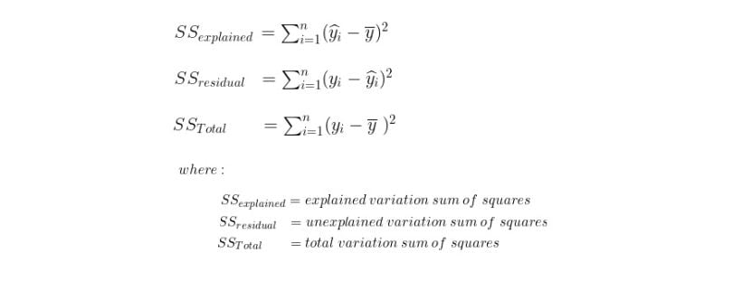
Here, we’ve calculated explained variation, unexplained variation and total variation of a single sample (row) of data. However, in the real world, we deal with multiple samples of data, so we need to calculate the squared variation of each sample and then compute the sum of those squared variations. This would give us a single number metric of variation. To achieve this, we need to slightly modify the formulae of the variations, as shown below.

What Is R-squared?

As we mentioned earlier, R-squared measures the variation that is explained by a regression model. The R-squared of a regression model is positive if the model’s prediction is better than a prediction, which is just the mean of the already available ‘y’ values. Otherwise, it’s negative. Below is the theoretical formula of R-squared.

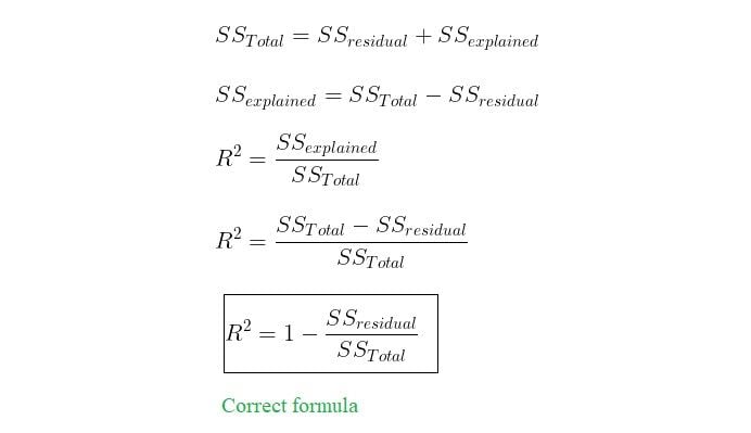
The formula is theoretically correct but only when the R-squared is positive. The formula doesn’t return a negative R-squared, as we are computing the sum of squares in both the numerator and denominator, which makes them always positive. As a result, it only returns a positive R-squared. We can derive the right formula (the one used in practice and also returns negative R-squared) from the above formula as shown below.

Let’s look at the implementation of R-squared in Python, compare it with Scikit-Learn’sr2_score() and see why the first formula is not always correct. For this, we’ll use the ‘Boston house prices’ data set of Scikit_Learn to fit a linear regression model. We’ll then create a function named my_r2_score() that computes the R-squared of the model.

import numpy as np
import pandas as pd
from sklearn.linear_model import LinearRegression
from sklearn.metrics import r2_score
from sklearn.datasets import load_boston

X = load_boston()['data'].copy()
y = load_boston()['target'].copy()

linear_regression = LinearRegression()
linear_regression.fit(X,y)

prediction = linear_regression.predict(X)

def my_r2_score(y_true, y_hat):
    y_bar = np.mean(y_true)
    ss_total = np.sum((y_true - y_bar) ** 2)
    ss_explained = np.sum((y_hat - y_bar) ** 2)
    ss_residual = np.sum((y_true - y_hat) ** 2)
    scikit_r2 = r2_score(y_true, y_hat)
    
    print(f'R-squared (SS_explained / SS_Total) = {ss_explained / ss_total}\n' + \
          f'R-squared (1 - (SS_residual / SS_Total)) = {1 - (ss_residual / ss_total)}\n'+ \
          f"Scikit-Learn's R-squared = {scikit_r2}")

print('Positive R-squared\n')
my_r2_score(y, prediction)

print('\n\nNegative R-squared\n')
my_r2_score(y, np.zeros(len(y)))

The output shows that the R-squared computed using the second formula is very similar to the result of Scikit-Learn’s r2-score() for both positive and negative R-squared values. However, as discussed earlier, the R-squared computed using the first formula is very similar to Scikit-Learn’s r2-score() only when the R-squared value is positive.

What Is Adjusted R-squared?

As we described earlier, R-squared increases or remains the same as we add new predictors to the multiple regression model. This remains the case even if the newly added predictors are independent of the target variable and don’t add any value to the predicting power of the model. Adjusted R-squared only increases if the newly added predictor improves the model’s predicting power. Adding independent and irrelevant predictors to a regression model results in a decrease of the adjusted R-squared.

Let’s look at how R-squared and adjusted R-squared behave upon adding new predictors to a regression model. We’ll use the ‘Boston house prices’ data set of Scikit-Learn. We’ll use the forward selection technique to build a regression model by incrementally adding one predictor at a time. Below are the steps we’ll follow.

1. Add three additional features named ‘random1’, ‘random2’ and ‘random3’ containing random numbers.
2. Calculate the mutual information scores of the features and incrementally add one feature at a time to the model in the decreasing order of the mutual information scores and compute the R-squared and adjusted R-squared.

import numpy as np
import pandas as pd
from sklearn.linear_model import LinearRegression
from sklearn.metrics import r2_score
from sklearn.datasets import load_boston
from sklearn.feature_selection import mutual_info_regression

df = pd.DataFrame(load_boston()['data'], columns=load_boston()['feature_names'])
df['y'] = load_boston()['target']

df['RAD'] = df['RAD'].astype('int')
df['CHAS'] = df['CHAS'].astype('int')

X = df.drop(columns='y').copy()
y = df['y'].copy()

np.random.seed(11)
X['random1'] = np.random.randn(len(X))
X['random2'] = np.random.randint(len(X))
X['random3'] = np.random.normal(len(X))

mutual_info = mutual_info_regression(X, y, discrete_features=X.dtypes == np.int32)
mutual_info = pd.Series(mutual_info, index=X.columns)
mutual_info.sort_values(ascending=False, inplace=True)
mutual_info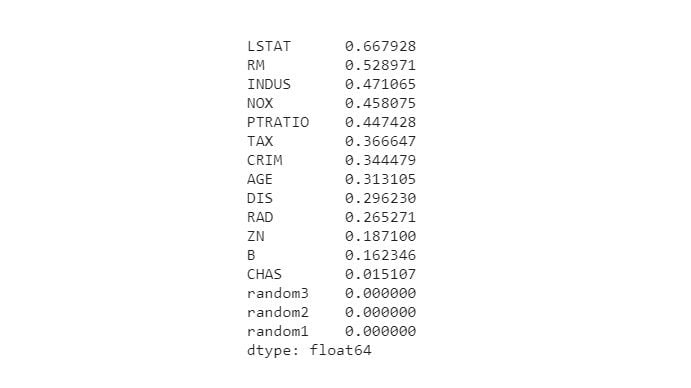

In the above mutual information scores, we can see that LSTAT has a strong relationship with the target variable and the three random features that we added have no relationship with the target. We’ll use these mutual information scores and incrementally add one feature at a time to the model (in the same order) and record the R-squared and adjusted R-squared scores.

result_df = pd.DataFrame()
for i in range(1, len(mutual_info) + 1):
    X_new = X.iloc[:, :i].copy()
    linear_regression = LinearRegression()
    linear_regression.fit(X_new, y)
    
    prediction = linear_regression.predict(X_new)
    r2 = r2_score(y_true=y, y_pred=prediction)
    adj_r2 = 1 - ((1 - r2) * (len(X) - 1) / (len(X) - i - 1))
    
    result_df = result_df.append(pd.DataFrame({'r2': r2,
                                              'adj_r2': adj_r2}, index=[i]))

result_df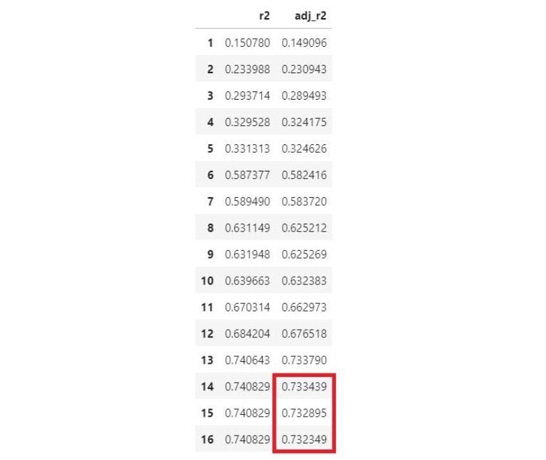

In the data frame, the index denotes the number of features added to the model. We can see a decrease in the adjusted R-squared as soon as we started adding the random features (the ones in the red box) to the model. However, R-squared remained the same.

Adjusted R-squared vs. R-Squared

R-squared measures the goodness of fit of a regression model. Hence, a higher R-squared indicates the model is a good fit, while a lower R-squared indicates the model is not a good fit. Below are a few examples of R-squared and the model fit.

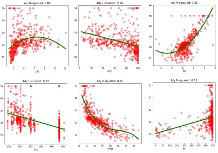
In the above plots, we can see that the models with a high adjusted R-squared seem to have a good fit compared to the ones with lower adjusted R-squared. However, this interpretation may not always hold up. Below are the two frequent questions asked by beginners regarding R-squared.

Is a High R-squared good?

If the training set’s R-squared is higher than the R-squared of the validation set, it indicates overfitting. If the same high R-squared translates to the validation set, then we can say that the model is a good fit.

More on Data Science: L1 and L2 Regularization Methods, Explained

Is a Low R-squared bad?

This depends on the type of the problem being solved. In some problems that are hard to model, an R-squared as low as 0.5 may be considered a good one. There is no rule of thumb that determines whether the R-squared is good or bad. However, a very low R-squared generally indicates underfitting, which means adding additional relevant features or using a complex model might help.

We’ve discussed the math behind R-squared and implemented it in Python. We’ve practically seen why adjusted R-squared is a more reliable measure of goodness of fit in multiple regression problems. We’ve discussed the way to interpret R-squared and found out the way to detect overfitting and underfitting using R-squared.