Gaussian Naive Bayes Explained With Scikit-Learn

Gaussian Naive Bayes (GNB) is a classification technique used in machine learning based on a probabilistic approach and Gaussian distribution. Gaussian Naive Bayes assumes that each parameter, also called features or predictors, has an independent capacity of predicting the output variable

The combination of the prediction for all parameters is the final prediction that returns a probability of the dependent variable to be classified in each group. The final classification is assigned to the group with the higher probability.

What Is Gaussian Distribution?

Gaussian distribution is also called normal distribution. Normal distribution is a statistical model that describes the distributions of continuous random variables in nature and is defined by its bell-shaped curve. The two most important features of the normal distribution are the mean (μ) and  standard deviation (σ). The mean is the average value of a distribution, and the standard deviation is the “width” of the distribution around the mean.

A variable (X) that is normally distributed is distributed continuously (continuous variable) from −∞ < X < +∞, and the total area under the model curve is 1.

More on AIHow to Develop Large Language Model (LLM) Applications

How to Use Gaussian Naive Bayes for Multi-Classification in Scikit-Learn

Gaussian Naive Bayes classification algorithm requires just a few steps to complete for multi-classification. Here’s how to do it yourself with sample code. 

1. Import the Libraries

The first step is to import the necessary libraries:

from random import random
from random import randint
import pandas as pd
import numpy as np
import seaborn as sns
import matplotlib.pyplot as plt
import statistics
from sklearn.model_selection import train_test_split
from sklearn.preprocessing import StandardScaler
from sklearn.naive_bayes import GaussianNB
from sklearn.metrics import confusion_matrix
from mlxtend.plotting import plot_decision_regions

2. Create a Database

Now, we will create a database in which the predictive variables are normally distributed.

#Creating values for FeNO with 3 classes:
FeNO_0 = np.random.normal(20, 19, 200)
FeNO_1 = np.random.normal(40, 20, 200)
FeNO_2 = np.random.normal(60, 20, 200)
#Creating values for FEV1 with 3 classes:
FEV1_0 = np.random.normal(4.65, 1, 200)
FEV1_1 = np.random.normal(3.75, 1.2, 200)
FEV1_2 = np.random.normal(2.85, 1.2, 200)
#Creating values for Broncho Dilation with 3 classes:
BD_0 = np.random.normal(150,49, 200)
BD_1 = np.random.normal(201,50, 200)
BD_2 = np.random.normal(251, 50, 200)
#Creating labels variable with three classes:(2)disease (1)possible disease (0)no disease:
not_asthma = np.zeros((200,), dtype=int)
poss_asthma = np.ones((200,), dtype=int)
asthma = np.full((200,), 2, dtype=int)
#Concatenate classes into one variable:
FeNO = np.concatenate([FeNO_0, FeNO_1, FeNO_2])
FEV1 = np.concatenate([FEV1_0, FEV1_1, FEV1_2])
BD = np.concatenate([BD_0, BD_1, BD_2])
dx = np.concatenate([not_asthma, poss_asthma, asthma])
#Create DataFrame:
df = pd.DataFrame()
#Add variables to DataFrame:
df['FeNO'] = FeNO.tolist()
df['FEV1'] = FEV1.tolist()
df['BD'] = BD.tolist()
df['dx'] = dx.tolist()
#Check database:
df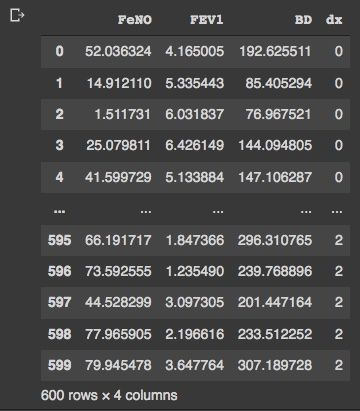

3. Check the Distribution of Variables

We have our data frame with 600 rows and four columns. Now, we can check the distribution of our variables by visual inspection:

fig, axs = plt.subplots(2, 3, figsize=(14, 7))
sns.kdeplot(df['FEV1'], shade=True, color="b", ax=axs[0, 0])
sns.kdeplot(df['FeNO'], shade=True, color="b", ax=axs[0, 1])
sns.kdeplot(df['BD'], shade=True, color="b", ax=axs[0, 2])
sns.distplot( a=df["FEV1"], hist=True, kde=True, rug=False, ax=axs[1, 0])
sns.distplot( a=df["FeNO"], hist=True, kde=True, rug=False, ax=axs[1, 1])
sns.distplot( a=df["BD"], hist=True, kde=True, rug=False, ax=axs[1, 2])
plt.show()

4. Build QQ-Plots to Double-Check Gaussian Distribution

By visual inspection, our data seems to be close to the Gaussian distribution. We can double-check building qq-plots:

from statsmodels.graphics.gofplots import qqplot
from matplotlib import pyplot
#q-q plot:
fig, axs = pyplot.subplots(1, 3, figsize=(15, 5))
qqplot(df['FEV1'], line='s', ax=axs[0])
qqplot(df['FeNO'], line='s', ax=axs[1])
qqplot(df['BD'], line='s', ax=axs[2])
pyplot.show()

5. Build a Pair-Plot to Explore the Data Set 

We don’t have a perfect normal distribution for our variables, but we are close enough and able to use them. To explore our data set and the correlations between variables, we will build a pair-plot:

#Exploring dataset:
sns.pairplot(df, kind="scatter", hue="dx")
plt.show()

6. Create a Box-Plot to Check Parameters

Next we’ll build a boxplot graph to check the distributions for the three groups and see which parameters best distinguish the categories:

# plotting both distibutions on the same figure
fig, axs = plt.subplots(2, 3, figsize=(14, 7))
fig = sns.kdeplot(df['FEV1'], hue= df['dx'], shade=True, color="r", ax=axs[0, 0])
fig = sns.kdeplot(df['FeNO'], hue= df['dx'], shade=True, color="r", ax=axs[0, 1])
fig = sns.kdeplot(df['BD'], hue= df['dx'], shade=True, color="r", ax=axs[0, 2])
sns.boxplot(x=df["dx"], y=df["FEV1"], palette = 'magma', ax=axs[1, 0])
sns.boxplot(x=df["dx"], y=df["FeNO"], palette = 'magma',ax=axs[1, 1])
sns.boxplot(x=df["dx"], y=df["BD"], palette = 'magma',ax=axs[1, 2])
plt.show()

How to Use Gaussian Naive Bayes in Scikit-Learn for Normal Distribution

Normal distribution has a mathematical equation that defines the probability of one observation of being in one of the groups. The formula is:

Where μ is mean and σ is standard deviation.

We can create a function to compute this probability:

#Creating a Function:
def normal_dist(x , mean , sd):
      prob_density = (1/sd*np.sqrt(2*np.pi)) * np.exp(-0.5*((x-mean)/sd)**2)
      return prob_density

If we know the normal distribution formula, we can manually compute the probability of observation to be in one of the three groups. First, we need to compute the mean and standard deviation for all predictive parameters and groups:

#Group 0:
group_0 = df[df['dx'] == 0]
print('Mean FEV1 group 0: ', statistics.mean(group_0['FEV1']))
print('SD FEV1 group 0: ', statistics.stdev(group_0['FEV1']))
print('Mean FeNO group 0: ', statistics.mean(group_0['FeNO']))
print('SD FeNO group 0: ', statistics.stdev(group_0['FeNO']))
print('Mean BD group 0: ', statistics.mean(group_0['BD']))
print('SD BD group 0: ', statistics.stdev(group_0['BD']))
#Group 1:
group_1 = df[df['dx'] == 1]
print('Mean FEV1 group 1: ', statistics.mean(group_1['FEV1']))
print('SD FEV1 group 1: ', statistics.stdev(group_1['FEV1']))
print('Mean FeNO group 1: ', statistics.mean(group_1['FeNO']))
print('SD FeNO group 1: ', statistics.stdev(group_1['FeNO']))
print('Mean BD group 1: ', statistics.mean(group_1['BD']))
print('SD BD group 1: ', statistics.stdev(group_1['BD']))
#Group 2:
group_2 = df[df['dx'] == 2]
print('Mean FEV1 group 2: ', statistics.mean(group_2['FEV1']))
print('SD FEV1 group 2: ', statistics.stdev(group_2['FEV1']))
print('Mean FeNO group 2: ', statistics.mean(group_2['FeNO']))
print('SD FeNO group 2: ', statistics.stdev(group_2['FeNO']))
print('Mean BD group 2: ', statistics.mean(group_2['BD']))
print('SD BD group 2: ', statistics.stdev(group_2['BD']))

Now, using an example observation with:

• FEV1 = 2.75
• FeNO = 27
• BD = 125

#Probability for:
#FEV1 = 2.75
#FeNO = 27
#BD = 125
#We have the same number of observations, so the general probability is: 0.33
Prob_geral = round(0.333, 3)
#Prob FEV1:
Prob_FEV1_0 = round(normal_dist(2.75, 4.70, 1.08), 10)
print('Prob FEV1 0: ', Prob_FEV1_0)
Prob_FEV1_1 = round(normal_dist(2.75, 3.70, 1.13), 10)
print('Prob FEV1 1: ', Prob_FEV1_1)
Prob_FEV1_2 = round(normal_dist(2.75, 3.01, 1.22), 10)
print('Prob FEV1 2: ', Prob_FEV1_2)
#Prob FeNO:
Prob_FeNO_0 = round(normal_dist(27, 19.71, 19.29), 10)
print('Prob FeNO 0: ', Prob_FeNO_0)
Prob_FeNO_1 = round(normal_dist(27, 42.34, 19.85), 10)
print('Prob FeNO 1: ', Prob_FeNO_1)
Prob_FeNO_2 = round(normal_dist(27, 61.78, 21.39), 10)
print('Prob FeNO 2: ', Prob_FeNO_2)
#Prob BD:
Prob_BD_0 = round(normal_dist(125, 152.59, 50.33), 10)
print('Prob BD 0: ', Prob_BD_0)
Prob_BD_1 = round(normal_dist(125, 199.14, 50.81), 10)
print('Prob BD 1: ', Prob_BD_1)
Prob_BD_2 = round(normal_dist(125, 256.13, 47.04), 10)
print('Prob BD 2: ', Prob_BD_2)
#Compute probability:
Prob_group_0 = Prob_geral*Prob_FEV1_0*Prob_FeNO_0*Prob_BD_0
print('Prob group 0: ', Prob_group_0)
Prob_group_1 = Prob_geral*Prob_FEV1_1*Prob_FeNO_1*Prob_BD_1
print('Prob group 1: ', Prob_group_1)
Prob_group_2 = Prob_geral*Prob_FEV1_2*Prob_FeNO_2*Prob_BD_2
print('Prob group 2: ', Prob_group_2)

The results prove that our observation with the values FEV1 = 2.75, FeNO = 27, and BD = 125 has a higher probability of being in group two. While these steps are highly educational and great for learning, they are time-consuming. 

More on AIForward Chaining vs. Backward Chaining in Artificial Intelligence

Using Gaussian Naive Bayes in Scikit-Learn to Evaluate Normal Distribution

Fortunately, we have a much faster way to do it. We can use the Gaussian Naive Bayes from Scikit-Learn, which is similar to other classification algorithms in its implementation. We create X and y variables and perform train and test split:

#Creating X and y:
X = df.drop('dx', axis=1)
y = df['dx']
#Data split into train and test:
X_train, X_test, y_train, y_test = train_test_split(X, y, test_size=0.30)

We also need to transform or normalize our data with standard scalar function:

sc = StandardScaler()
X_train = sc.fit_transform(X_train)
X_test = sc.transform(X_test)

And now build and evaluate the model:

#Build the model:
classifier = GaussianNB()
classifier.fit(X_train, y_train)
#Evaluate the model:
print("training set score: %f" % classifier.score(X_train, y_train))
print("test set score: %f" % classifier.score(X_test, y_test))

We can visualize our results using a confusion matrix:

# Predicting the Test set results
y_pred = classifier.predict(X_test)
#Confusion Matrix:
cm = confusion_matrix(y_test, y_pred)
print(cm)

We can see by the confusion matrix that our model is best to predict class 0, but has a higher error rate with classes 1 and 2. Lastly, we can build decision boundaries graphs using two variables:

df.to_csv('data.csv', index = False)
data = pd.read_csv('data.csv')
def gaussian_nb_a(data):
    x = data[['BD','FeNO',]].values
    y = data['dx'].astype(int).values
    Gauss_nb = GaussianNB()
    Gauss_nb.fit(x,y)
    print(Gauss_nb.score(x,y))
    #Plot decision region:
    plot_decision_regions(x,y, clf=Gauss_nb, legend=1)
    #Adding axes annotations:
    plt.xlabel('X_train')
    plt.ylabel('y_train')
    plt.title('Gaussian Naive Bayes')
    plt.show()
def gaussian_nb_b(data):
    x = data[['BD','FEV1',]].values
    y = data['dx'].astype(int).values 
    Gauss_nb = GaussianNB()
    Gauss_nb.fit(x,y)
    print(Gauss_nb.score(x,y))
    #Plot decision region:
    plot_decision_regions(x,y, clf=Gauss_nb, legend=1)
    #Adding axes annotations:
    plt.xlabel('X_train')
    plt.ylabel('y_train')
    plt.title('Gaussian Naive Bayes') 
    plt.show()
def gaussian_nb_c(data):
    x = data[['FEV1','FeNO',]].values
    y = data['dx'].astype(int).values
    Gauss_nb = GaussianNB()
    Gauss_nb.fit(x,y)
    print(Gauss_nb.score(x,y))
    #Plot decision region:
    plot_decision_regions(x,y, clf=Gauss_nb, legend=1)
    #Adding axes annotations:  
    plt.xlabel('X_train')
    plt.ylabel('y_train')  
    plt.title('Gaussian Naive Bayes')
    plt.show()
gaussian_nb_a(data)
gaussian_nb_b(data)
gaussian_nb_c(data)

And that’s all there is to it!