Explaining the Empirical Rule for Normal Distribution

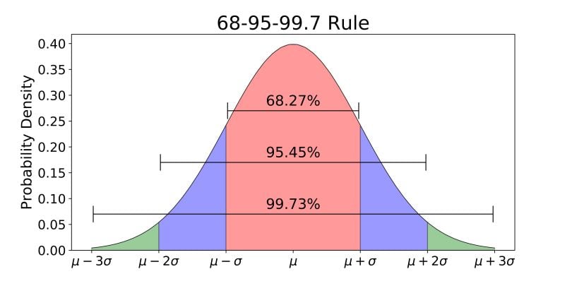
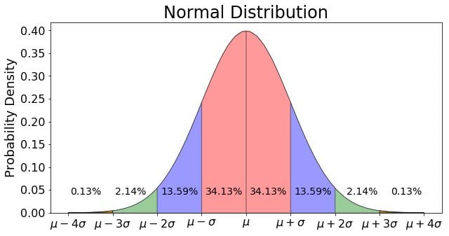
Normal distribution is commonly associated with the 68-95-99.7 rule, or empirical rule, which you can see in the image below. Sixty-eight percent of the data is within one standard deviation (σ) of the mean (μ), 95 percent of the data is within two standard deviations (σ) of the mean (μ), and 99.7 percent of the data is within three standard deviations (σ) of the mean (μ).

This post explains how those numbers were derived in the hope that they can be more interpretable for your future endeavors. 

As always, the code used to make everything — including the graphs — is available on my GitHub. With that, let’s get started.

Empirical Rule & the Probability Density Function

To understand where the 68-95-99.7 percentages come from, it’s important to first understand the probability density function, known as the PDF. A PDF is used to specify the probability of the random variable falling within a particular range of values, as opposed to taking on any one value. The integral of the variable’s PDF over the range gives its probability. 

That is, it’s given by the area under the density function but above the horizontal axis, and by the area between the lowest and greatest values of the range. This definition might not make much sense, so let’s graph the probability density function for a normal distribution to clear it up. The probability density function for a normal distribution is represented in the equation below:

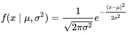
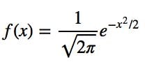
Let’s simplify it by assuming we have a mean (μ) of zero and a standard deviation (σ) of one.

Now that the function is simpler, let’s graph this function with a range from -3 to 3.

# Import all libraries for the rest of the blog post
from scipy.integrate import quad
import numpy as np
import matplotlib.pyplot as plt
from matplotlib.patches import Polygon
%matplotlib inline

x = np.linspace(-3, 3, num = 100)
constant = 1.0 / np.sqrt(2*np.pi)
pdf_normal_distribution = constant * np.exp((-x**2) / 2.0)
fig, ax = plt.subplots(figsize=(10, 5));
ax.plot(x, pdf_normal_distribution);
ax.set_ylim(0);
ax.set_title('Normal Distribution', size = 20);
ax.set_ylabel('Probability Density', size = 20);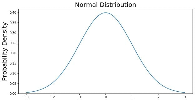

More on DataUnderstanding Train Test Split

How to Find the Probability of Events 

The graph above does not show you the probability of events but their probability density. We will need to integrate to get the probability of an event within a given range. Suppose we are interested in finding the probability of a random data point landing within one standard deviation of the mean. We need to integrate from -1 to 1. This can be done with SciPy.

# Make a PDF for the normal distribution a function
def normalProbabilityDensity(x):
   constant = 1.0 / np.sqrt(2*np.pi)
   return(constant * np.exp((-x**2) / 2.0) )

# Integrate PDF from -1 to 1
result, _ = quad(normalProbabilityDensity, -1, 1, limit = 1000)
print(result)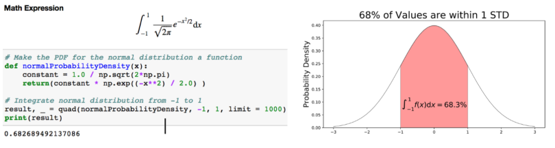

You’ll see that 68 percent of the data is within one standard deviation (σ) of the mean (μ).

If you are interested in finding the probability of a random data point landing within two standard deviations of the mean, you need to integrate from -2 to 2.

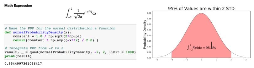
Now, 95 percent of the data is within two standard deviations (σ) of the mean (μ).

If you are interested in finding the probability of a random data point landing within three standard deviations of the mean, you need to integrate from -3 to 3.

And now, 99.7 percent of the data is within three standard deviations (σ) of the mean (μ).

It is important to note that for any probability density function, the area under the curve must be one. The probability of drawing any number from the function’s range is always one.

More on Data4 Probability Distributions Every Data Scientist Needs to Know

You will also find that it is also possible for observations to fall four, five or even more standard deviations from the mean, but this is very rare if you have a normal, or nearly normal, distribution.

You can now take this knowledge and apply it to boxplots.