Understanding Ordinary Least Squares (OLS) Regression

Ordinary least squares (OLS) regression is an optimization strategy that helps you find a straight line as close as possible to your data points in a linear regression model (known as a best-fit line). It works to minimize the sum of squared differences between the observed and predicted values in the model, with the best-fit line representing this minimization. OLS is considered one of the most useful optimization strategies for linear regression models as it can help you find unbiased real value estimates for your alpha (α) and beta (β) parameters.

Why is that? It’s helpful to first understand linear regression algorithms.

How OLS Applies to Linear Regression

Linear regression is a statistical method employed in supervised machine learning tasks to model the linear relationship between one dependent variable and one or more independent variables. In particular, it works to predict the value of a dependent variable based on the value of an independent variable.

Since supervised machine learning tasks are normally divided into classification and regression tasks, we can allocate linear regression algorithms into the regression category. It differs from classification because of the nature of the target variable. In classification, the target is a categorical value (“yes/no,” “red/blue/green,” “spam/not spam,” etc.). Regression involves numerical, continuous values as a target. As a result, the algorithm will be asked to predict a continuous number rather than a class or category. Imagine that you want to predict the price of a house based on some relative features, the output of your model will be the price, hence, a continuous number.

Regression tasks can be divided into two main groups: simple or linear regression (which uses only one independent variable to predict the target variable), and multiple regression (which uses more than one independent variable to predict the target variable). 

To give you an example, let’s consider the house task above. If you want to predict a house’s price only based on its squared meters, you will fall into the first situation (one feature), but if you are going to predict the price based on its squared meters, its position and the liveability of the surrounding environment, you are going to fall into the second group for multiple features.

In the first scenario, you are likely to employ a simple linear regression algorithm, which we’ll explore more later in this article. On the other hand, whenever you’re facing more than one feature to explain the target variable, you are likely to employ a multiple linear regression.

Simple linear regression is a statistical model widely used in machine learning regression tasks. It’s based on the idea that the relationship between two variables can be explained by the following formula:

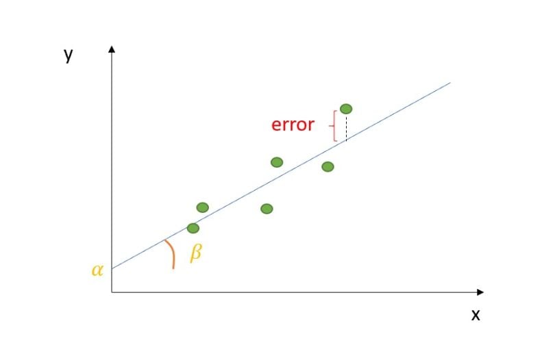
Where εi is the error term, and α, β are the true (but unobserved) parameters of the regression. The parameter β represents the variation of the dependent variable when the independent variable has a unitary variation. If my parameter is equal to 0.75, when my x increases by one, my dependent variable will increase by 0.75. On the other hand, the parameter α represents the value of our dependent variable when the independent one is equal to zero.

Let’s visualize it graphically:

More on Machine Learning: What Is Unsupervised Learning?

How to Find OLS in a Linear Regression Model

The goal of simple linear regression is to find the parameters α and β for which the error term is minimized. To be more precise, the model will minimize the squared errors. Indeed, we don’t want our positive errors to be compensated for by the negative ones, since they are equally penalizing our model.

This procedure is called ordinary least squares (OLS) error.

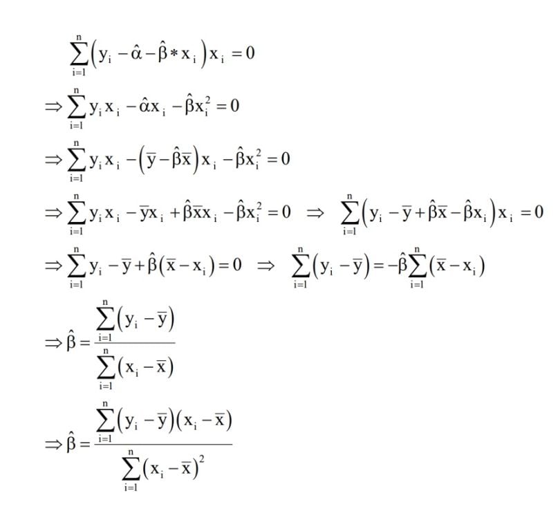
Let’s demonstrate those optimization problems step-by-step. If we reframe our squared error sum as follows:

We can set our optimization problem as follows:

So, let’s start with β:

Knowing that the sample covariance between two variables is given by:

And that the sample correlation coefficient between two variables is equal to:

We can reframe the above expression as follows:

The same reasoning holds for our α:

Once obtained, those values of α and β, which minimize the squared errors, our model’s equation will look like this:

More on Machine Learning: Multiclass Classification With an Imbalanced Data Set

Advantages of OLS Regression

Think of OLS as an optimization strategy to obtain a straight line from your model that is as close as possible to your data points. 

Even though OLS is not the only linear regression optimization strategy, it’s  commonly used for these tasks since the outputs of the regression (coefficients) are unbiased estimators of the real values of alpha and beta. OLS regression’s simplicity and computational efficiency as a linear regression optimization technique also lends to its popularity.

Indeed, according to the Gauss-Markov Theorem, under some assumptions of the linear regression model (linearity in parameters, random sampling of observations, conditional mean equal to zero, absence of multicollinearity and homoscedasticity of errors), the OLS estimators α and β are the best linear unbiased estimators (BLUE) of the real values of α and β​.

Limitations of OLS Regression

Despite its popular applications in linear regression models, OLS regression can have some drawbacks.

For one, OLS regression is sensitive to outliers in data, such as extremely large or small values for the dependent variable in comparison to the rest of the data set. Since OLS focuses on minimizing the sum of squared errors, outliers can disproportionately affect model results.

OLS also assumes linearity in data and attempts to fit data to a straight line, though this may not always reflect the complexities of relationships between values in real life. For example, OLS can attempt to apply a best-fit line to curved or non-linear data points, leading to inaccurate model results.

Additionally, the OLS algorithm can become less effective as more features (independent variables) are added to the model. When a large number of independent variables are added — where the number of features is more than the number of data points — errors are more likely to occur and the OLS solution may not be unique.

Frequently Asked Questions