

Dimensionality reduction is the process of transforming high-dimensional data into a lower-dimensional format while preserving its most important properties. This technique is used in machine learning and has applications in many industries including quantitative finance, healthcare and drug discovery. The applications of dimensionality reduction are numerous and can be either supervised or unsupervised. Every data scientist should know some state-of-the-art methods for carrying it out.
What Is Dimensionality Reduction?
Supervised vs. Unsupervised Dimensionality Reduction
Dimensionality reduction methods fall into two categories: supervised and unsupervised, depending on the availability of data labels.
In supervised dimensionality reduction, the data includes labeled outcomes, meaning that each input has a known result to predict. Methods that use supervised reduction aim to find a reduced set of features relevant to the defined task or target variable. Random forests are a common method of supervised dimensionality reduction. They use a machine learning algorithm that creates many decision trees for classification and regression tasks. Each decision tree asks yes or no questions about the values in the data and successively splits them into similar groups based on the answer.
In contrast, unsupervised dimensionality reduction works with data that has no labeled outcomes. Dimensionality techniques that use unsupervised reduction work best with complex data sets, as they transform data into smaller sets of uncorrelated variables while maintaining essential features. Principal component analysis, PCA, is one of the most common unsupervised dimensionality reduction methods.
How to Prepare Data for Dimensionality Reduction in Python
Let’s start by importing the Pandas library:
import pandas as pd We then can relax the display limits for rows and columns:
pd.set_option('display.max_columns', None)
pd.set_option('display.max_rows', None)
Next, let’s read our data into a Pandas data frame:
df = pd.read_csv()Let’s see how many columns and rows are in our data:
print("Number of Columns: ", len(list(df.columns)))
print("Number of rows: ", len(df))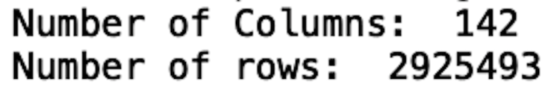
We see that we have 142 columns and 2.9 million rows. This is a pretty large data set to work with on most machines, so it’s a great candidate for dimensionality reduction.
Now, let’s display the first five rows of the data. Since this data set is relatively large, the columns are truncated in the screenshot below. When you run this code locally on your machine you will be able to see all of the columns:
print(df.head())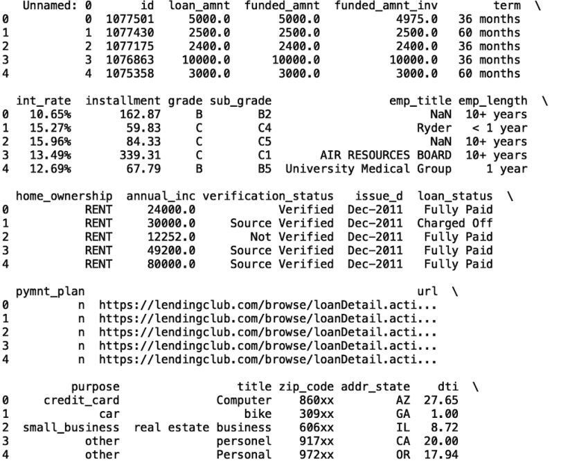
Working with a data set of this size on a local machine can be cumbersome. As you’ll notice when you run this code, simple tasks such as reading in the data and displaying take quite some time. Thus, we’ll consider only a subset of the data in our analysis — credit card repayment loans. This corresponds to the purpose column with the value of credit_card. Let’s filter our data to only have credit card repayment loans.
df = df[df['purpose'] == 'credit_card']Let’s also take a small subset of the columns. We’ll consider the following fields in the data:
columns = ['loan_amnt', 'loan_status','funded_amnt',
'funded_amnt_inv', 'term',
'int_rate','mths_since_recent_revol_delinq','home_ownership',
'verification_status',
 'num_accts_ever_120_pd', 'num_actv_bc_tl',
'num_actv_rev_tl', 'avg_cur_bal', 'bc_open_to_buy', 'bc_util',
'chargeoff_within_12_mths', 'delinq_amnt', 'last_fico_range_low',
'last_fico_range_high']

df = df[columns]
For details on what each of these fields mean, see the data dictionary. Some important fields are loan amount, interest rates, home ownership status, FICO scores, and number of active accounts.
Now, let’s also write the filtered data frame to a new csv file that we will call credit_card_loans.csv:
df.to_csv("credit_card_loan.csv", index=False)Now, let’s read in our new csv file into a separate data frame. We will call this new dataframe df_credit:
df_credit = pd.read_csv("credit_card_loan.csv")Now, let’s print the new number of rows and columns:
print("Number of Columns: ", len(list(df_credit.columns)))
print("Number of rows: ", len(df_credit))
We see that our data now has 18 columns and 695,665 rows. This size set is significantly easier to work with.
Next, let’s print the first five rows of data:
print(df_credit.head())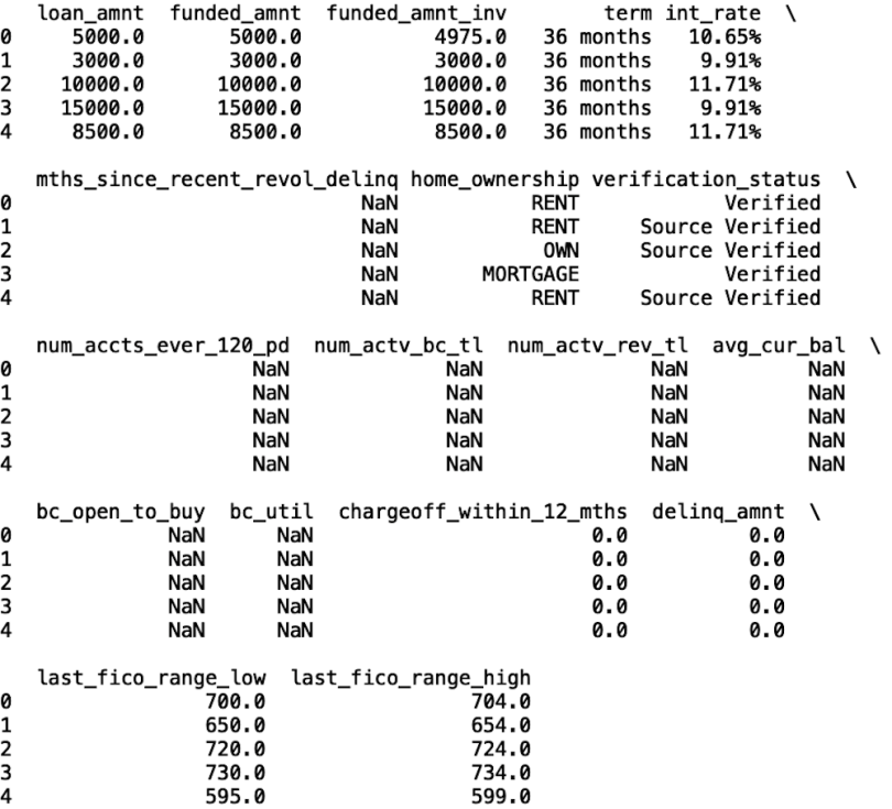
Before we discuss any specific methods, note that we were already able to significantly reduce the dimensionality of the data in terms of both columns and rows. But we still need to do a bit more data prep. Notice some columns have missing values — NaN means not a number. Let’s impute those with the mean for each of these columns:
def fill_na(numerical_column):
df_credit[numerical_column].fillna(df_credit[numerical_column].mean(), inplace=True)

fill_na('mths_since_recent_revol_delinq')
fill_na('num_accts_ever_120_pd')
fill_na('num_actv_bc_tl')
fill_na('num_actv_rev_tl')
fill_na('avg_cur_bal')
fill_na('bc_open_to_buy')
fill_na('bc_util')

print(df_credit.head())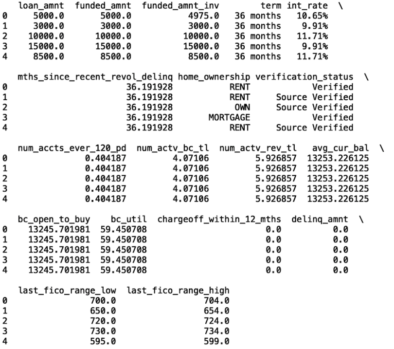
We see the missing values have been imputed. Next, let’s convert the categorical columns into codes that are machine-readable. This conversion is necessary when using most machine learning packages available in Python:
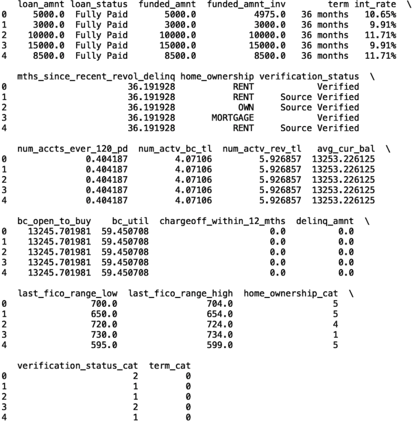
Now, the home ownership, term and verification status columns have corresponding categorical columns. The first method we’ll look at is using random forests feature importance to reduce dimensionality. This is a supervised machine learning method since random forests require labeled data.
So, the next thing we need to do is generate labels from the loan_status columns. First, let’s print the unique set of values for loan status:
print(set(df_credit[‘loan_status’]))
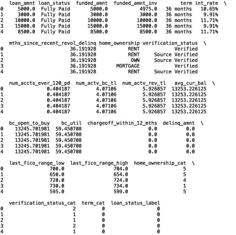
For simplicity, let’s only consider the loan status outcomes fully paid and default/charged off. We will also combine these.
df_credit = df_credit[df_credit['loan_status'].isin(['Fully Paid',
'Default', 'Charged Off'])]
Let’s also create binary labels for these loan status outcomes. A value of one will correspond to default/charged off, meaning the loan wasn’t paid off and has gone into collections. Zero means the loan was paid in full.
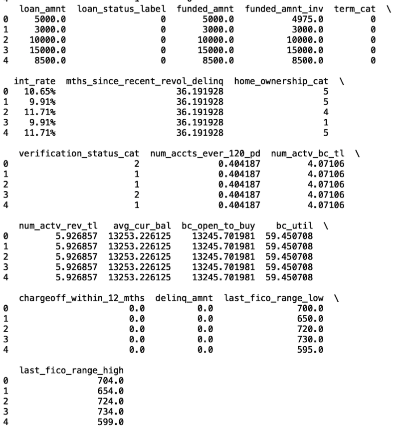
Finally, let’s filter the columns in our data frame so we only have columns with machine-readable values.
columns2 = ['loan_amnt', 'loan_status_label', 'funded_amnt',
'funded_amnt_inv', 'term_cat',
'int_rate','mths_since_recent_revol_delinq','home_ownership_cat',
'verification_status_cat',
 'num_accts_ever_120_pd', 'num_actv_bc_tl', 'num_actv_rev_tl',
'avg_cur_bal', 'bc_open_to_buy', 'bc_util',
'chargeoff_within_12_mths', 'delinq_amnt', 'last_fico_range_low',
'last_fico_range_high']
df_credit = df_credit[columns2]
print(df_credit.head())
Finally, let’s convert the interest rate column into a numerical column:
df_credit['int_rate'] = df_credit['int_rate'].str.rstrip('%')
df_credit['int_rate'] = df_credit['int_rate'].astype(float)
df_credit.fillna(0, inplace=True)
How to Use Random Forests for Dimensionality Reduction
Now we’re in good shape to apply random forests, which is a tree-based ensemble algorithm that constructs a series of tree data structures and asks yes-or-no questions about the statistics in the data. Each of these trees makes a prediction based on the answers, and the trees are combined to make a single prediction. Let’s import the random forest classifier and the train/test split methods from Scikit-learn.
from sklearn.ensemble import RandomForestClassifier
from sklearn.model_selection import train_test_split
Let’s define our input and output and split our data for training and testing. This step is necessary so that we don’t overfit to noise in our training data and ensures that our model can generalize well when we make predictions on future data.
X = df_credit[['loan_amnt', 'funded_amnt', 'funded_amnt_inv',
'term_cat', 'int_rate','mths_since_recent_revol_delinq','home_ownership_cat', 'verification_status_cat',
 'num_accts_ever_120_pd', 'num_actv_bc_tl', 'num_actv_rev_tl',
'avg_cur_bal', 'bc_open_to_buy', 'bc_util',
'chargeoff_within_12_mths', 'delinq_amnt', 'last_fico_range_low',
'last_fico_range_high']]
y = df_credit['loan_status_label']

X_train, X_test, y_train, y_test = train_test_split(X, y ,
random_state=42, test_size = 0.33)
Next, let’s fit our random forest model to the training data and generate a plot for feature importance.
import seaborn as sns
import matplotlib.pyplot as plt
model = RandomForestClassifier()
model.fit(X_train, y_train)

features = ['loan_amnt', 'funded_amnt', 'funded_amnt_inv', 'term_cat', 'int_rate','mths_since_recent_revol_delinq','home_ownership_cat',
'verification_status_cat',
 'num_accts_ever_120_pd', 'num_actv_bc_tl', 'num_actv_rev_tl',
'avg_cur_bal', 'bc_open_to_buy', 'bc_util',
'chargeoff_within_12_mths', 'delinq_amnt', 'last_fico_range_low',
'last_fico_range_high']


feature_df = pd.DataFrame({"Importance":model.feature_importances_,
"Features": features })
sns.set()
plt.bar(feature_df["Features"], feature_df["Importance"])
plt.xticks(rotation=90)
plt.title("Random Forest Model Feature Importance")
plt.show()
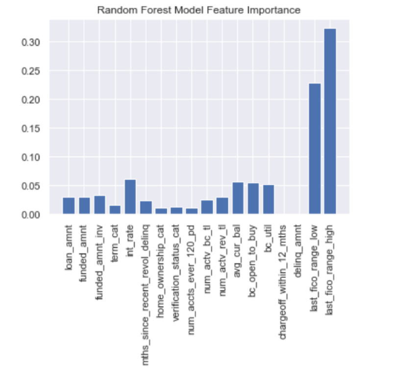
We see that the FICO scores, interest rate and current balance are the three most important features. We can clearly use the random forest feature importance to narrow down which factors to consider when predicting credit risk.
The downside with this method is that it assumes we have labels. In this case, it’s loan status. Often, though, we can find use cases in which we’d like to narrow down a large list of columns in data without having any labels. The most common technique for this approach is principal component analysis.
What Is PCA and How Is It Used for Dimensionality Reduction?
Principal component analysis works by finding a smaller set of column values from an uncorrelated larger set. This method works by representing independent, uncorrelated features as a sum of the original features.
Let’s start by importing the PCA package from Sklearn. We will also need the StandardScaler method from the preprocessing module in Sklearn.
from sklearn.decomposition import PCA
from sklearn.preprocessing import StandardScaler
Now, let’s define the input for our PCA algorithm.
X = df_credit[features2]Next, let’s scale our data using the standardScaler method. This step helps with numerical stability when the algorithm computes the components.
scaler = StandardScaler()
X_scaled = scaler.fit(X)
Next, let’s define a PCA object with four components, fit to X_scaled, then generate our components.
pca=PCA(n_components=4)
pca.fit(X_scaled)
X_components=pca.transform(X_scaled)
We can then store the component in a Pandas data frame.
components_df = pd.DataFrame({'component_one':
list(X_components[:,0]), 'component_two': list(X_components[:,1]),
                              'component_three':
list(X_components[:,2]), 'component_four': list(X_components[:,3])})

print(components_df.head())

Now, we’ll store the class in a variable called labels and define some variables that we’ll use for formatting our plot:
labels=X.loan_status_label
color_dict={0:'Red',1:'Blue'}
fig,ax=plt.subplots(figsize=(7,5))
sns.set()
We can now generate our scatter plot and add axes labels and a title. We will look at a scatter plot of the first two components:
for i in np.unique(labels):
index=np.where(labels==i)   ax.scatter(components_df['component_one'].loc[index],components_df['component_two'].loc[index],c=color_dict[i],s=10,
           label=i)


plt.xlabel("1st Component",fontsize=14)
plt.ylabel("2nd Component",fontsize=14)
plt.title('Scatter plot of Principal Components')
plt.legend()
plt.show()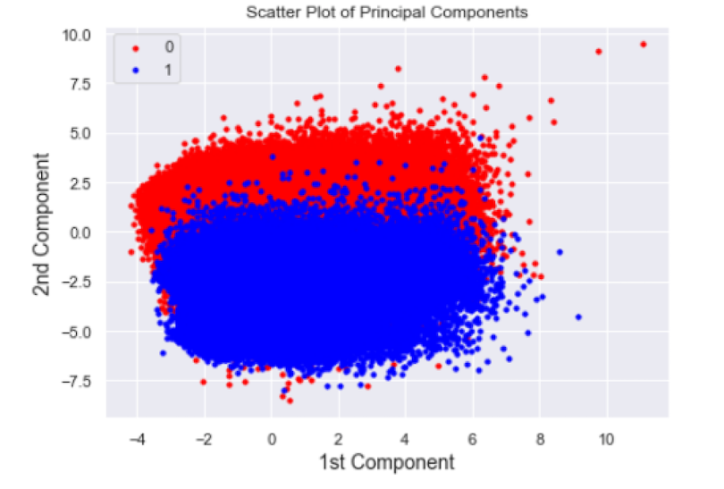
We can see a distinct separation between classes in our scatter plot. Although we have labels that we can use for a sanity check for our PCA algorithm, in practice, PCA is used in an unsupervised manner. This means we can use these methods to explore distinct clusters for any column we are interested in.
For example, we can explore clusters in credit scores or even income. Cluster analysis of these values may be useful for lenders because it allows them to consider creditworthy borrowers who would otherwise be denied a loan. An example is a recent graduate student with a low credit score who recently got a job in the tech industry with a high-six-figure salary. While the borrower was in graduate school, they may have had trouble paying off loans, but they may now be creditworthy upon starting their new job.
This type of cluster analysis can help detect these borrowers who would otherwise be denied for a loan which can translate to higher revenue for lenders. PCA is very powerful in this sense since it can allow you to analyze distinct groups in your data without requiring any predefined labels.
The code in this post is available on GitHub.
Dimensionality Reduction in Python: The Takeaway
Most data science teams across industries are faced with the task of reducing the dimensionality of data. This may be for the sake of simple analytics, building interpretable models or even performing cluster analysis on a large data set. Random forest is useful for dimensionality reduction when you have a well-defined supervised learning problem. In our case, our labels were credit default and fully paid off loans. Random forest is also appealing because you can directly interpret how significant the features used in your model are for determining an outcome. PCA is a powerful tool when you do not have labels in your data. Companies can use PCA to explore distinct groups in data which can then be used to make decisions.
Frequently Asked Questions
What is dimensionality reduction?
Dimensionality reduction is a data science technique that transforms high-dimensional data into a lower-dimensional format while preserving the most important features. It helps make complex datasets more manageable.
What is dimensionality reduction in machine learning?
Dimensionality reduction is used in machine learning to simplify models, reduce computation requirements and overfitting, a scenario where AI struggles with unseen data.
What are 3 ways of reducing dimensionality?
There are several methods to reduce dimensionality but most can be divided into feature selection and feature extraction categories. The three most common methods of reducing dimensionality include:
- Principal component analysis (PCA): a feature extraction technique that identifies principal components and transforms them into uncorrelated variables that retain its variance data.
- Linear discriminant analysis (LDA): a supervised reduction method that finds linear combinations of features to separate data into different classes.
- Singular value decomposition (SVD): a dimensionality reduction technique that decomposes a data matrix into three matrices. It is used in natural language processing and recommendation systems.
Is PCA dimensionality reduction?
Yes, principal component analysis, or PCA, is a widely used method for dimensionality reduction. PCA transforms high-dimensional data sets into a lower-dimensional space and retains as much data variance as possible.
What is the difference between PCA and LDA and SVD?
PCA, LDA and SVD are all dimensionality reduction techniques, but they differ in their purpose and application.
- PCA: an unsupervised technique that reduces dimensionality by finding the principle components and variance in a dataset.
- LDA: a supervised technique that separates data into differentiating classes.
- SVD: an unsupervised technique that decomposes a data matrix into three matrices.
What is an example of dimensionality reduction in real life?
A real life example of dimensionality reduction is facial recognition systems. A photo of a face contains thousands of pixels and identifiable features. Using dimensionality reduction, facial recognition systems are able to reduce the number of features while maintaining the ones used to match an image to a person.


