A Guide to Outlier Detection in Python

Outlier detection, also known as anomaly detection, is a common task for many data science teams. It is the process of identifying data points that have extreme values compared to the rest of the distribution.

Benefits of Outlier Detection

Outlier detection has a wide range of applications including data quality monitoring, identifying price arbitrage in finance, detecting cybersecurity attacks, healthcare fraud detection, banknote counterfeit detection and more. 

In each of these applications, outliers correspond to events that are rare or uncommon. For example, in the case of cybersecurity attacks, most of the events represented in the data will not reflect an actual attack. Only a small fraction of the data will indicate bona fide cyberattacks. 

Similarly, with counterfeit banknote detection, the majority of the records will represent authentic banknotes, while the counterfeit banknotes will make up a small fraction of the total data. The task of outlier detection is to quantify common events and use them as a reference for identifying relative abnormalities in data. 

Methods for Outlier Detection in Python

For outlier detection, Python offers a variety of easy-to-use methods and packages. Before selecting a method, however, you need to first consider modality. This is the number of peaks contained in a distribution.

For example, imagine that you have a data column composed of athletes’ weights. If the data is multimodal, there are many highly dense regions in the distribution. This can mean that there are many athletes with weights between 200 and 210 pounds and a comparable number of athletes between 230 and 240 pounds.

In addition to modality, when considering methods for outlier detection, you should consider data set size and dimensionality, meaning the number of columns. If your data is relatively small, say a few dozen features and a few thousand rows, simple statistical methods such as box plot visualizations should suffice. If your data is moderately sized and multimodal (meaning there are many peaks), isolation forests are a better choice. If your data is high dimensional, large and multimodal, OneClassSVM may be a better choice.

Here we will be using various methods to address the task of identifying counterfeit banknotes using the Swiss banknote counterfeit detection data set. 

More From Sadrach PierreA Guide to Selecting Machine Learning Models in Python

Prerequisite to Outlier Detection: Reading in Data

To start practicing outlier detection on the Python data set, let’s import the Pandas library, which is used for reading in, transforming and analyzing data. We will use Pandas to read our data into a data frame:

import pandas as pd 

df = pd.read_csv("banknotes.csv")

Next, let’s display the first five rows of data using the .head() method:

print(df.head())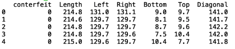

Here we see that the data contains the columns length, left, right, bottom, top and diagonal, which all correspond to the dimensions of the banknotes in millimeters. We also see a counterfeit column that has ground truth values indicating whether the bank note is counterfeit or authentic. A value of one corresponds to counterfeit and a value of zero means authentic. 

Using Box Plots for Outlier Detection 

A box plot is a standard way to visualize outliers and the quartiles for numerical values in data. Quartiles divide numerical data into four groups:

1. The first quartile is the middle number between the minimum and the median, so 25 percent of the data falls below this point.

2. The second quartile is the median, which means that 50 percent of the data falls below this point.

3. The third quartile is the middle number between the maximum and the median, so 75 percent of the data falls below this point. 

4. The fourth quartile is the highest 25 percent of the data 

Let’s look at the box plot for the length column. To do this, let’s import Seaborn and use the box plot method. Let’s also import Matplotlib, which we will use to title our box plot:

import seaborn as sns
import matplotlib.pyplot as plt
sns.boxplot(data=df,x=df["Length"])
plt.title("Boxplot of Swiss Banknote Length ")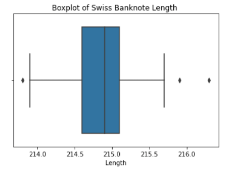

The dots in the box plots correspond to extreme outlier values. We can validate that these are outlier by filtering our data frame and using the counter method to count the number of counterfeits:

df_outlier1 = df[df['Length']> 216].copy()
print(Counter(df_outlier1['conterfeit']))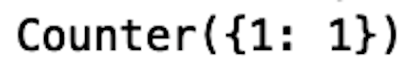

We see that, with these conditions, we only capture one out of every 100 counterfeit banknotes. If we relax the filtering conditions to capture additional outliers, we’ll see that we also capture authentic banknotes as well:

df_outlier2 = df[df['Length']> 215.5].copy()
print(Counter(df_outlier2['conterfeit']))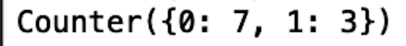

This corresponds to a precision of 0.30, which isn’t a great performance. Even worse, this corresponds to an accuracy of 1.5 percent. 

To help address this inaccuracy, we can look at box plots for additional columns. Let’s create box plots for the remaining columns and a function that allows us to generate box plots for any numerical column:

def boxplot(column):
    sns.boxplot(data=df,x=df[f"{column}"])
    plt.title(f"Boxplot of Swiss Banknote {column}")
    plt.show()

And let’s call the function with the columns length, left, right, bottom, top and diagonal:

boxplot('Length')
boxplot('Right')
boxplot('Left')
boxplot('Bottom')
boxplot('Top')
boxplot('Diagonal')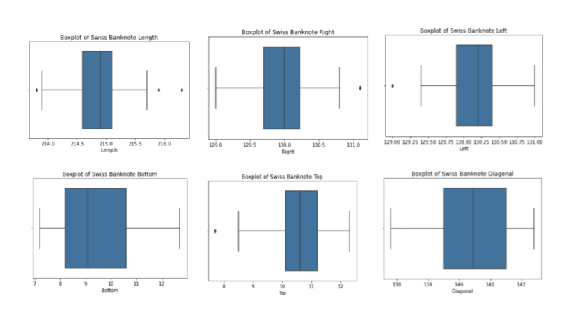

We can filter on the top 50 percent for length, right, left and bottom:

df_outlier3 = df[(df['Length']> 215)&(df['Right']> 130)&(df['Left']> 
130)&(df['Bottom']> 10)].copy()
print(Counter(df_outlier3['conterfeit']))

We see that we now capture eight counterfeits. Although this is an improvement on the single counterfeit banknote we captured before, we still missed 92 additional counterfeits, which corresponds to an accuracy of four percent. Further, the more numerical columns we have in our data the more cumbersome the task of outlier detection becomes. For this reason, box plots are ideal for small and simple data sets with few columns. 

Using Isolation Forests for Outlier Detection 

An isolation forest is an outlier detection method that works by randomly selecting columns and their values in order to separate different parts of the data. It works well with more complex data, such as sets with many more columns and multimodal numerical values. 

Let’s import the IsolationForest package and fit it to the length, left, right, bottom, top and diagonal columns. Notice that this algorithm only takes inputs because it’s an unsupervised machine learning technique, unlike supervised machine learning techniques, which are trained on both features and targets. Luckily, we can still validate our predictions because our data comes with the counterfeit labels.

First, let’s import the necessary packages:

from sklearn.ensemble import IsolationForest
from sklearn.model_selection import train_test_split
from sklearn.metrics import precision_score
import numpy as np

Next, let’s define our input and output (we will only use this for validation, not training), and split our data:

X = df[['Length', 'Left', 'Right', 'Bottom', 'Top', 'Diagonal']]
y = df['conterfeit']
X_train, X_test, y_train, y_test = train_test_split(X, y, 
test_size=0.33, random_state=42)

Next, let’s fit our model to our inputs:

clf = IsolationForest(random_state=0)
clf.fit(X_train)
y_pred = clf.predict(X_test)

Finally, let’s predict the test data and evaluate the precision score. Again, in practice, since this is unsupervised machine learning, we wouldn’t have labels to validate our models. For our purposes here, though, we will validate so we have a sense how well the methods can detect outliers:

pred = pd.DataFrame({'pred': y_pred})
pred['y_pred'] = np.where(pred['pred'] == -1, 1, 0)
y_pred = pred['y_pred'] 
print("Precision:", precision_score(y_test, y_pred))

We see that our outlier detection model has a precision of 0.625. Compare this to the precision of 0.30 we achieved with the box plots. This model also gives an accuracy of 56 percent, compared to the four percent from box plots, which shows a significant improvement in outlier detection. This is because isolation forests are able to partition the data and identify outliers along multiple features.

When we use box plots we have to manually inspect outliers and try to draw conclusions using multiple features, which becomes increasingly difficult the greater the number of features. For example, you can have a cluster of points where individual feature values may not be outliers, but a combination of values may be anomalous. This type of behavior is difficult to detect through inspecting box plots. 

More in Data ScienceBaffled by Covariance vs. Correlation? You’re Not Alone.

Using OneClassSVM for Outlier Detection 

Now, let’s explore how to use OneClassSVM for outlier detection. This is another unsupervised machine learning technique that is useful for high dimensional and large data sets. Let’s import the necessary packages, fit our model and evaluate the performance:

clf_svm = OneClassSVM(gamma='auto')
clf_svm.fit(X_train)
y_pred_svm = clf_svm.predict(X_test)

pred['svm'] = y_pred_svm
pred['svm_pred'] = np.where(pred['svm'] == -1, 1, 0)

y_pred_svm = pred['svm_pred']
print("SVM Precision:", precision_score(y_test, y_pred_svm))

We see that our precision decreases compared to the isolation forest method. Our accuracy also decreases from 56 percent to 47 percent when we compare isolation forests to OneClassSVM. This is likely because our data is relatively small and low-dimensional and our model overfit the data. This means that the algorithm models random noise and fluctuations in the data that don’t correspond to discernable patterns.

In this case, this random noise that the model learns fails to help capture the separation between outliers and inliers, meaning the normal data points. The tendency of OneClassSVM to overfit explains the decrease in performance compared to isolation forest.

The code from this post is available on GitHub. 

Master Outlier Detection

Although we looked at methods for solving the task of outlier detection for identifying counterfeit banknotes, these methods can be applied to a wide variety of outlier detection tasks. For example, box plots can carry out tasks such as credit card fraud detection. Isolation forests are useful for tasks such as defected item detection in manufacturing. OneClassSVM applies to tasks that involve high dimensional data such as detecting bullying or terrorist activity using social media text data.

Whether you are working with financial data, manufacturing data or social media data, having a decent knowledge of outlier detection tools is useful for any data scientist. Although we only considered tabular numerical data, the basic concept of outlier detection applies across use cases. This article can serve as the foundation for data scientists just starting out learning outlier detection techniques in Python. These easy-to-use packages can help data scientists solve a variety of common outlier detection problems which translates to added value for clients, data science teams and companies overall.