Mean Squared Error (MSE) vs. Mean Squared Logarithmic Error (MSLE): A Guide

Mean squared error (MSE) and mean squared logarithmic error (MSLE) are two loss functions that can significantly impact the results of your analyses. While MSE is one of the most common loss functions, it has some lesser known drawbacks. It works well with continuous targets, but it has some quirks with data in the 0 to 1 territory. Large outliers can also severely influence the loss, drawing away the focus.

On the other hand, MSLE isn’t used as often as MSE, but it solves some of the shortcomings MSE has by utilizing the traits of a logarithm. Log transformation reduces disparity between large and small values, giving them more equal weight. However, those outliers might be important to you. 

A supervised machine learning problem in statistical terms is all about predicting a target variable based on a set of features, or independent variables. This prediction is judged based on a loss function, a metric quantifying how close your predicted values are to the actual target variable values. And this is not only important in terms of evaluation, during model training, a lot of decisions are taken automatically based on this loss (or objective) function. Selecting the right loss function is a critical choice to make, and one that practitioners often overlook despite its significance.

RelatedHow Loss Functions Work in Neural Networks and Deep Learning

What Is Mean Squared Error (MSE)?

A popular option for model optimziation is to use mean squared error (MSE). This involves minimizing the average of the squared errors, or taking the mean of the squared differences between predicted and actual values.

How to Calculate MSE

In Python, you’re most likely going to use the sklearn.metrics.mean_squared_error function. This function will take the actual true y values and your predicted ones, and it will return the value of the loss function.

If you want to calculate it from scratch, you are going to need the formula:

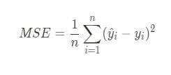
To calculate it, you’ll subtract the predicted values from the actual target values, square those differences 1-1 and then take the mean of the resulting squared error array.

import numpy as np

actual = np.array([1, 2, 3, 4, 5])
predicted = np.array([1.1, 1.9, 2.7, 4.5, 6])

def mse(actual: np.ndarray, predicted: np.ndarray) -> float:
    differences = np.subtract(actual, predicted)
    squared_differences = np.square(differences)
    return np.mean(squared_differences)

mse(actual, predicted)
# 0.27199999999999996

When to Use MSE

The main thing you have to consider when deciding your loss function is how your target variable looks, and what error distribution you would tolerate more. 

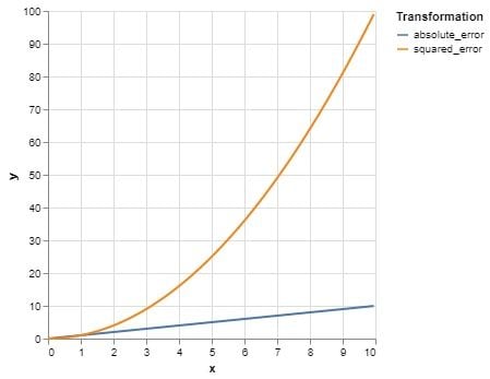
Squaring errors in MSE amplifies large differences and preserves the impact of small ones (such as those under a value of 1), making the model more sensitive to large deviations between predicted and actual values.

This means large errors drive the loss, shifting model focus toward higher-value targets.

In summary, you should consider mean squared error if:

• You are doing a baseline analysis before making any decisions.
• You have some star performers, and you are the most keen on making a good model for those.
• Your data is predominantly in the same order of magnitude.

What Is Mean Squared Logarithmic Error (MSLE)?

Mean squared logarithmic error (MSLE) is a less commonly used loss function. It’s considered to be an improvement over using percentage based errors for training because its numerical properties are better, but it essentially serves the same purpose: Trying to create a balance between data points with orders of magnitude difference during model training.

How to Calculate MSLE

In Python, you most probably are going to use sklearn.metrics.mean_squared_logarithmic_error, which works exactly like the MSE counterpart.

To calculate it from scratch, use the formula: 

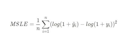
You have to add one to the actual and predicted target values (adding one ensures that all inputs to the logarithm are greater than zero, preventing undefined values and maintaining numerical stability), and take their differences by subtracting the latter from the former. 

Then, we square those logarithmic differences 1-1, then take the mean.

import numpy as np

actual = np.array([1, 2, 3, 4, 5])
predicted = np.array([1.1, 1.9, 2.7, 4.5, 6])

def msle(actual: np.ndarray, predicted: np.ndarray) -> float:
    log_differences = np.subtract(np.log(1 + actual), np.log(1 + predicted))
    squared_log_differences = np.square(log_differences)
    return np.mean(squared_log_differences)

msle(actual, predicted)

When to Use MSLE

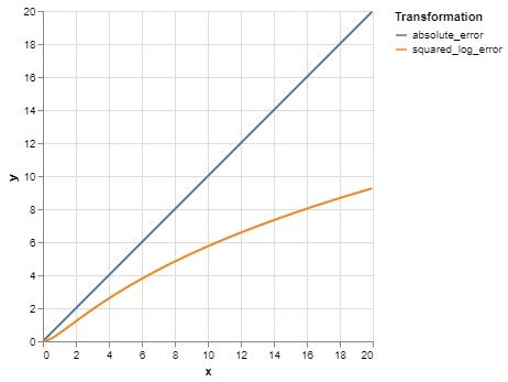
MSLE essentially makes the error profile more flat, reducing the impact of the larger values. 

Additionally, some workflows use the square root of MSLE (RMSLE) for more interpretable results, especially when reporting errors in the same units as the target variable.

It’s important to note that this metric assumes non-negative target variables. As a result, the previously seen overwhelming effect of large values is reduced, producing a more equal emphasis on data points.

In summary, you should use MSLE if:

• You want to level the playing field for target values that differ by several orders of magnitude.
• You aim for a balanced model having roughly similar percentage errors.
• You can tolerate large differences in terms of units for large target values.

RelatedL1 and L2 Regularization, Methods Explained

How to Select the Best Loss Function for Your Model

The loss function you select can have a significant impact on the model you’re building. 

Imagine that you’re working for a supermarket chain, and you want to predict the sales for individual products in its various points of sale. Most likely, sales distribution data will be skewed. Some stores will sell orders of magnitude more than others, and the same would apply to products. As a result, your target variable will have a power law distribution. To make matters worse, products have different shelf lives. So, to make a fair comparison, one might consider daily average sold quantities.

A well-known trick is to take the natural logarithm of the values, which forces the distribution to be closer to normal, in order to transform the target variable. Still, you’re dealing with a target variable with vast differences.

In these situations, the loss function you optimize for greatly influences your predictions. One might aim for the predictions to be in a certain percentile range of your targets. You could argue that “My predictions are in the ‘+-x% range’ of the sales numbers.” On the other hand, you might aim for actual sales number precision, as in, “My predictions are right with ‘x unit’ precision.” On top of that, you need to decide on whether you want to focus your predictions on the stores with lower revenue or the fewer high-achiever stores. These tradeoffs are mostly determined by which loss function you choose for your statistical model. 

So, how do you select the right loss function model?

Mean Squared Error (MSE) vs. Mean Squared Logarithmic Error (MSLE)

Let’s use the above example and run a quick simulation predicting the sales of individual products for the next period, using sales data from the current (previous) period as a feature. We’ll look at two models, one that’s trained with mean squared error (MSE) and the other mean squared logarithmic error (MSLE). The bars show the percentage difference between the results of the two models in terms of their respective error bases.

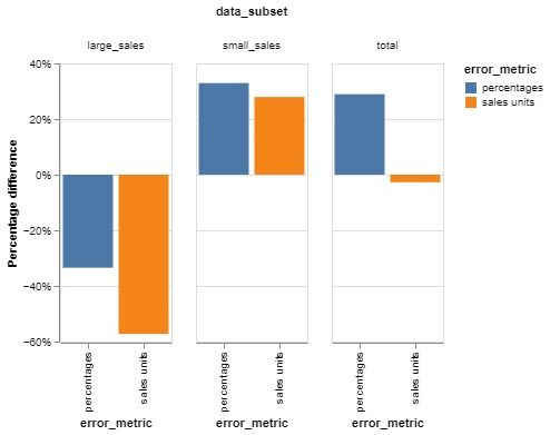
Looking at the graph, the negative percentage differential shows that the MSE model is more effective in that particular segment, producing smaller errors, while the positive differential indicates that the MSLE model is performing better for that group. 

For instance, the first bar group shows large sales places/products. The MSE objective model has a 30 percent better percentage error and is 56 percent better when errors are measured in sales units. On the other hand, when looking at small sales, the MSLE model is better in terms of units and percentages.

The same phenomenon can be seen on the third bar group. 

Percentage-wise, MSLE performs better because of the better percentage errors it produces for small sales, which make up most of the data. MSLE tends to approximate relative error more closely than MSE, making it more suitable when percentage-based accuracy is a higher priority. Also, MSLE inherently penalizes underpredictions more than overpredictions, which can lead to a systematic bias toward underestimating target values.

Meanwhile, MSLE optimization results in large errors in sales units for large sales, effectively making MSE a slightly better performer in terms of units over the whole group. 

So, what should you learn from all of this? In my view, these are the most important takeaways from this chart:

1.  MSE trained models perform better on large sales occasions. These are generally fewer but might be more important. In contrast, MSLE performs better for the average, small sales stores.
2. In all data subsets, MSLE models provide an improvement if errors are measured in percentages. The same applies for MSE if the errors are in sales units.
3. Always consider the loss function you want to optimize for in your use case. Don’t just go with the default one.

Frequently Asked Questions