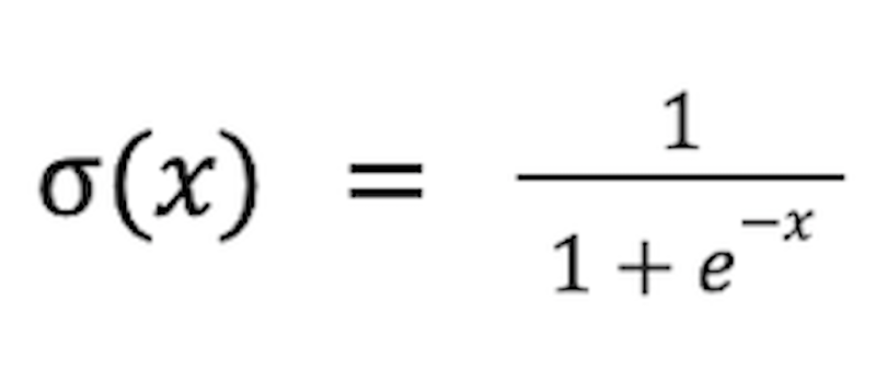
The sigmoid is used as a neural network activation function and is defined by the following formula:
It’s characterized by a gradual rise from zero, followed by a relatively rapid increase before it levels off near one, as shown in the following graph:
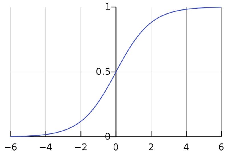
We’ll dig into more specifics later.
What Is the Sigmoid Activation Function?
The sigmoid activation function has applications to machine learning through its operations in neural networks. Briefly, you can think of each layer in a neural network as a matrix that takes in an input vector and produces an output vector. The whole network is formed by chaining such matrix multiplications together. In machine learning, an activation function applies some non-linear function after each matrix multiplication so the network can learn any necessary functional relationship and not just linear ones.
Why Is the Sigmoid Function Important?
The importance of the sigmoid is to some degree historical. It’s one of the earliest activation functions that was used in neural networks. But what exactly are activation functions? Briefly, you can think of each layer in a neural network as a matrix that takes in an input vector and produces an output vector. The whole network is formed by chaining such matrix multiplications together.
Just composing matrices isn’t enough, however. If we used only matrix multiplications, then our network could only ever represent linear functions, but we want it to learn any necessary functional relationship. To allow for this, we must apply some non-linear function after each matrix multiplication. That’s what an activation function does.
Neural networks initially took inspiration from the brain, where neurons behave in a binary fashion: Either they fire or they don’t. Inspired by this, we might try applying an activation function that transforms a vector to be just zeroes and ones. We need our activation function to be smooth in order to apply backpropagation and learn, however. Technically, we require that the function be differentiable. To differentiate a function means to find its slope at each point. For a function to be differentiable, it must have a well-defined slope at each point. Non-differentiable functions have either sudden jumps or sharp turns.
A true binary activation function like this wouldn’t even be continuous, so it won’t work for our purposes. A continuous function is one with no sudden jumps. All differentiable functions have to be continuous. A binary activation function would have to jump straight from zero to one at some point as we adjust the input, and hence is not continuous.
This principle is what motivates the sigmoid function. It’s a smooth version of our idea above. It maps most inputs to be either very close to zero or very close to one, while still being differentiable.
The sigmoid has some inefficiencies, which we’ll discuss, that have reduced its usage in more recent years. But it still plays a central role in binary classification, which we’ll also discuss. For now, let’s dig more into the function itself.
Sigmoid Activation Function Formula
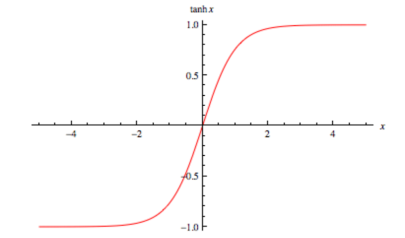
First, we should clear up some terminological confusion. Technically speaking, a “sigmoid” is any S-shaped curve that flattens out near its minimum and maximum values. For example, the hyperbolic tangent (tanh) is technically a sigmoid function:
In modern machine learning parlance, however, “sigmoid activation function” typically refers specifically to the logistic sigmoid function:
From here on out, when we say “sigmoid,” we just mean the logistic function. Its equation is:
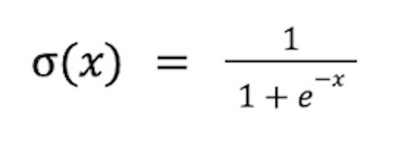
As we said before, it’s differentiable, non-linear, has a range from zero to one, and squishes most values toward the minimum or maximum.
Components of Function
The input to the sigmoid is given by the value x. The exponential term in the denominator means that as x gets large, e-x shrinks rapidly, approaching zero. Thus, the whole function quickly approaches one. Conversely, for small x (i.e., large negative x), e-x grows rapidly, approaching infinity. In this case, the whole function swiftly converges to zero.
If you have some mathematical expertise, you may be aware that the exponential function ex is approximately linear for small values of x. This is why the sigmoid looks almost like a straight line around x=0, but rapidly approaches zero or one as we move further away.
The mathematically inclined may also know that ex is particularly easy to differentiate, the derivative of ex being ex itself. This ease carries over to the sigmoid. Its derivative is also very simple to compute:
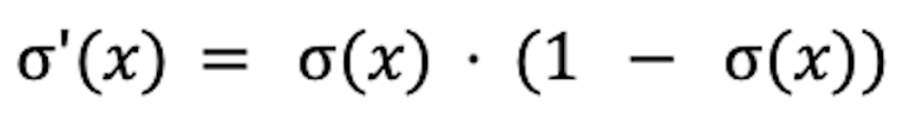
This is convenient since, to train a neural network, we must know how changing the network weights will affect the final output. The slope (or rate of change) of the activation function is critical for calculating this, and it’s easy to determine for the sigmoid.
Applications of Function
The sigmoid can be used simply as an activation function throughout a neural network, applying it to the outputs of each network layer. It isn’t used as much nowadays, however, because it has a couple of inefficiencies.
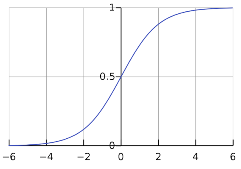
The first is the problem of saturating gradients. Looking at its graph, we can see that the sigmoid has a strong slope in the middle, but at the ends, its slope is very shallow. This is a problem for learning. At a high level, when we run gradient descent, many of the neurons in our network will be outputting values in the shallow regions of the sigmoid. Changing the network weights will then have little effect on its overall output, and learning comes to a halt.
In a little more detail, to run backpropagation and learn, we must take the gradient of the loss function with respect to each parameter in our network. At first, some neurons may be outputting values in the middle of the sigmoid range, where the slope is strong. But as we make updates, we move up or down this slope and quickly end up in a shallow region. The magnitude of our gradient then becomes smaller and smaller, meaning we take smaller and smaller learning steps. Learning is not very efficient this way.
The other problem with the sigmoid is that it’s not symmetric about the origin. In the brain, neurons either fire or don’t, so we may have the intuition that neuron activations should be zero or one. Despite this, researchers have actually found that neural networks learn better when activations are centered around zero. This is one of the reasons it’s a good idea to standardize your data (i.e., shift it to have mean zero) before feeding it into a neural network. It’s also one of the reasons for batch normalization, a similar process where we standardize our network activations at intermediate layers rather than just at the start.
If you look at the beginning of the previous section, you’ll see that the tanh function ranges from -1 to one and is centered around zero. For this reason, it’s often preferable to the sigmoid. It also has the problem of saturating gradients, though. The most common activation function nowadays is the rectified linear unit (ReLU):
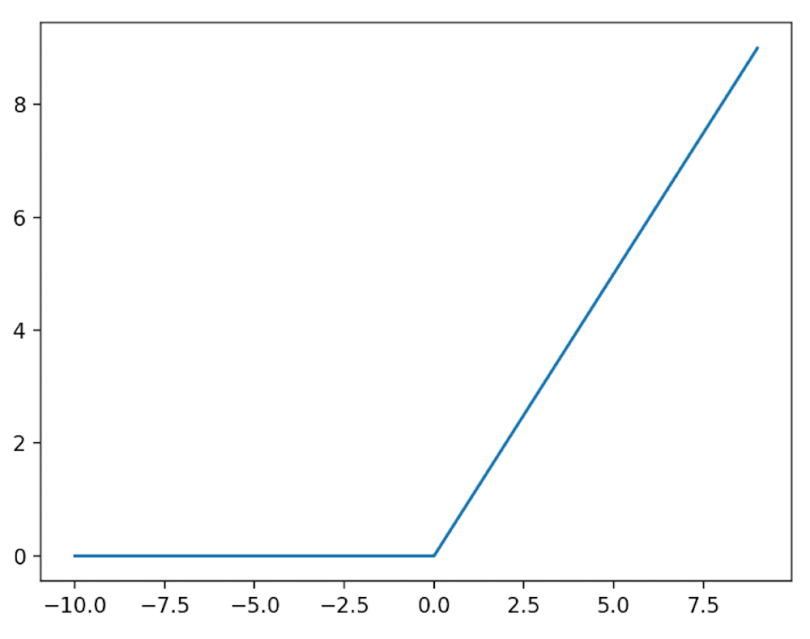
This function has a strong slope everywhere to the right of zero, although it’s obviously not symmetric around zero. So, tanh has saturating gradients, and ReLU is non-symmetric. In practice, the former is a bigger problem than the latter. The moral here, though, is that the sigmoid is the worst of both worlds on these fronts.
Despite all this, the sigmoid still has a place in modern machine learning: binary classification. In binary classification, we categorize inputs as one of two classes. If we’re using neural networks, the output of our network must be a number between zero and one, representing the probability that the input belongs to class one (with the probability for class two being immediately inferable).
The output layer of such a network consists of a single neuron. Consider the output value of this neuron. Before applying any activation function, it can be any real number, which is no good. If we apply a ReLU, it will be positive (or zero). If we use tanh, it will be between -1 and one. None of these work. We must apply a sigmoid to this last neuron. We need a number between zero and one, and we still need the activation function to be smooth for the purposes of training. The sigmoid is the right choice.
In these cases, we can still use some other activation function for the earlier layers in the network. It’s only at the very end that we need the sigmoid. The use of sigmoid in this way is still absolutely standard in machine learning and is unlikely to change anytime soon. Thus, the sigmoid lives on!