Machine Learning Basics Every Beginner Should Know

Machine learning is an application of artificial intelligence where a machine learns from past experiences (input data) and makes future predictions. It’s typically divided into three categories: supervised learning, unsupervised learning and reinforcement learning.

This article introduces the basics of machine learning theory, laying down the common concepts and techniques involved. This post is intended for people starting with machine learning, making it easy to follow the core concepts and get comfortable with machine learning basics.

What Is Machine Learning?

In 1959, Arthur Samuel, a computer scientist who pioneered the study of artificial intelligence, described machine learning as “the study that gives computers the ability to learn without being explicitly programmed.”

Alan Turing’s seminal paper introduced a benchmark standard for demonstrating machine intelligence, such that a machine has to be intelligent and responsive in a manner that cannot be differentiated from that of a human being.

A more technical definition given by Tom M. Mitchell’s 1997 paper: “A computer program is said to learn from experience E with respect to some class of tasks T and performance measure P, if its performance at tasks in T, as measured by P, improves with experience E.” For example, a handwriting recognition learning problem:

• Task T: Recognizing and classifying handwritten words within images.
• Performance measure P: Percent of words correctly classified, accuracy.
• Training experience E: A data-set of handwritten words with given classifications.

In order to perform the task T, the system learns from the data set provided. A data set is a collection of many examples. An example is a collection of features.

More on Machine LearningAll Machine Learning Models Explained

Common Types of Machine Learning 

Machine learning is generally categorized into three types: Supervised learning, unsupervised learning, reinforcement learning.

Supervised Learning

In supervised learning the machine experiences the examples along with the labels or targets for each example. The labels in the data help the algorithm to correlate the features.

Two of the most common supervised machine learning tasks are classification and regression.

In classification, the machine learning model takes in data and predicts the most likely category, class or label it belongs to based on its values. Some examples of classification include predicting stock prices and categorizing articles to news, politics or leisure based on its content.

In regression, the machine predicts the value of a continuous response variable. Common examples include predicting sales of a new product or a salary for a job based on its description.

Unsupervised Learning

When we have unclassified and unlabeled data, the system attempts to uncover patterns from the data . There is no label or target given for the examples. One common task is to group similar examples together called clustering.

Reinforcement Learning

Reinforcement learning refers to goal-oriented algorithms, which learn how to attain a complex objective (goal) or maximize along a particular dimension over many steps. This method allows machines and software agents to automatically determine the ideal behavior within a specific context in order to maximize its performance. Simple reward feedback is required for the agent to learn which action is best. This is known as the reinforcement signal. For example, maximizing the points won in a game over a lot of moves.

Supervised Machine Learning Techniques

Regression is a technique used to predict the value of response (dependent) variables from one or more predictor (independent) variables.

Most commonly used regressions techniques are linear regression and logistic regression. We will discuss the theory behind these two prominent techniques alongside explaining many other key concepts like gradient descent algorithm, overfit and underfit, error analysis, regularization, hyperparameters and cross validation techniques involved in machine learning.

Linear Regression

In linear regression problems, the goal is to predict a real-value variable y from a given pattern X. In the case of linear regression the output is a linear function of the input. Let ŷ be the output our model predicts: ŷ = WX+b

Here X is a vector or features of an example, W are the weights or vector of parameters that determine how each feature affects the prediction, and b is a bias term. So, our task T is to predict y from X. Now ,we need to measure performance P to know how well the model performs.

To calculate the performance of the model, we first calculate the error of each example i as:

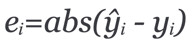
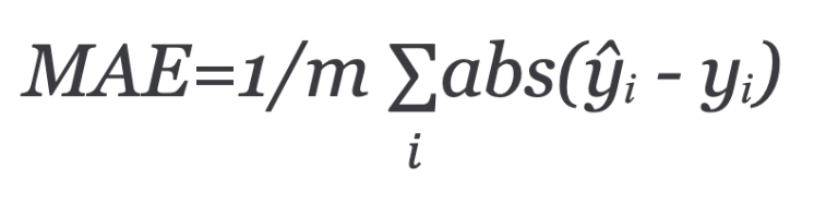
We then take the absolute value of the error to take into account both positive and negative values of error. Finally, we calculate the mean for all recorded absolute errors  or the average sum of all absolute errors.

Mean absolute error (MAE) equals the average of all absolute errors:

A more popular way of measuring model performance is using Mean squared error (MSE). This is the average of squared differences between prediction and actual observation.

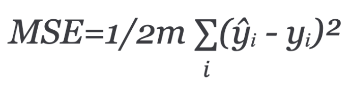
The mean is halved as a convenience for the computation of the gradient descent, as the derivative term of the square function will cancel out the half term. 

The main aim of training the machine learning algorithm is to adjust the weights W to reduce the MAE or MSE.

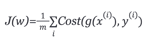
To minimize the error, the model updates the model parameters W while experiencing the examples of the training set. These error calculations when plotted against the W is also called cost function J(w), since it determines the cost/penalty of the model. So, minimizing the error is also called as minimizing the cost function J.

Gradient Descent Algorithm:

In the gradient descent algorithm, we start with random model parameters and calculate the error for each learning iteration, keep updating the model parameters to move closer to the values that results in minimum cost.

Repeat until minimum cost: 

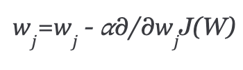
In the above equation, we are updating the model parameters after each iteration. The second term of the equation calculates the slope or gradient of the curve at each iteration.

The gradient of the cost function is calculated as a partial derivative of cost function J with respect to each model parameter wj, where j takes the value of number of features [1 to n]. α, alpha, is the learning rate, or how quickly we want to move towards the minimum. If α is too large, we can overshoot. If α is too small, it means small steps of learning, which increases the overall time it takes the model to observe all examples.

There are three ways of doing gradient descent:

1. Batch gradient descent: Uses all of the training instances to update the model parameters in each iteration.
2. Mini-batch gradient descent: Instead of using all examples, mini-batch gradient descent divides the training set into smaller size called batch denoted by ‘b’. Thus a mini-batch ‘b’ is used to update the model parameters in each iteration.
3. Stochastic gradient descent (SGD): This updates the parameters using only a single training instance in each iteration. The training instance is usually selected randomly. Stochastic gradient descent is often preferred to optimize cost functions when there are hundreds of thousands of training instances or more, as it will converge more quickly than batch gradient descent.

Logistic Regression

In some problems the response variable isn’t normally distributed. For instance, a coin toss can result in two outcomes: heads or tails. The Bernoulli distribution describes the probability distribution of a random variable that can take the positive case with probability P or the negative case with probability 1-P. If the response variable represents a probability, it must be constrained to the range {0,1}.

In logistic regression, the response variable describes the probability that the outcome is the positive case. If the response variable is equal to or exceeds a discrimination threshold, the positive class is predicted. Otherwise, the negative class is predicted.

The response variable is modeled as a function of a linear combination of the input variables using the logistic function.

Since our hypotheses ŷ has to satisfy 0 ≤ ŷ ≤ 1, this can be accomplished by plugging logistic function or sigmoid function:

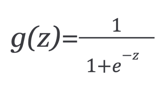
The function g(z) maps any real number to the (0, 1) interval, making it useful for transforming an arbitrary-valued function into a function better suited for classification. 

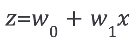
Now, coming back to our logistic regression problem, let’s assume that z is a linear function of a single explanatory variable x. We can then express z as follows:

And the logistic function can now be written as:

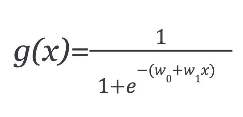
g(x) is interpreted as the probability of the dependent variable. g(x) = 0.7, gives us a probability of 70 percent that our output is one. Our probability that our prediction is zero is just the complement of our probability that it is one. For example, if the probability that it’s one is 70 percent, then the probability that it is zero is 30 percent.

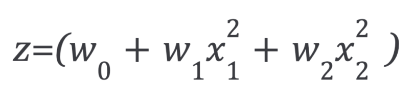
The input to the sigmoid function g doesn’t need to be a linear function. It can be a circle or any shape.

Cost Function

We cannot use the same cost function that we used for linear regression because the sigmoid function will cause the output to be wavy, causing many local optima. In other words, it will not be a convex function.

In order to ensure the cost function is convex, and therefore, ensure convergence to the global minimum, the cost function is transformed using the logarithm of the sigmoid function. The cost function for logistic regression looks like:

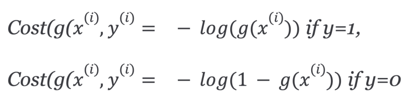
Which can be written as:

So, the cost function for logistic regression is:

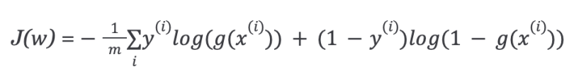
Since the cost function is a convex function, we can run the gradient descent algorithm to find the minimum cost.

What Is Underfitting and Overfitting in Machine Learning?

We try to make the machine learning algorithm fit the input data by increasing or decreasing the model’s capacity. In linear regression problems, we increase or decrease the degree of the polynomials.

Consider the problem of predicting y from x ∈ R. Since the data doesn’t lie in a straight line, the fit is not very good.

To increase model capacity, we add another feature by adding the term x² to it. This produces a better fit. But if we keep on doing so x⁵, fifth order polynomial), we may be able to better fit the data but it will not generalize well for new data.

Underfitting

When the model has fewer features, it isn’t able to learn from the data very well.  This means the model has a high bias.

Overfitting

When the model has complex functions, it’s able to fit the data but is not able to generalize to predict new data. This model has high variance. There are three main options to address the issue of overfitting:

1. Reduce the number of features: Manually select which features to keep. We may miss some important information if we throw away features.
2. Regularization: Keep all the features, but reduce the magnitude of weights W. Regularization works well when we have a lot of slightly useful features.
3. Early stopping: When we are training a learning algorithm iteratively such as using gradient descent, we can measure how well each iteration of the model performs. Up to a certain number of iterations, each iteration improves the model. After that point, however, the model’s ability to generalize can weaken as it begins to overfit the training data.

Regularization in Machine Learning

Regularization can be applied to both linear and logistic regression by adding a penalty term to the error function in order to discourage the coefficients or weights from reaching large values.

Linear Regression With Regularization

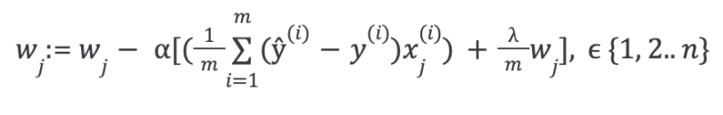
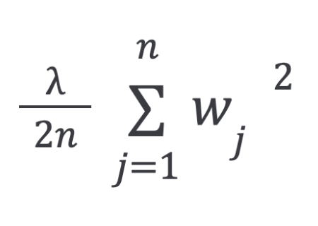
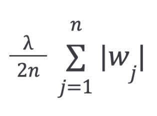
The simplest such penalty term takes the form of a sum of squares of all of the coefficients, leading to a modified linear regression error function:

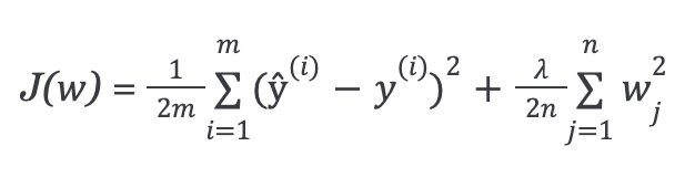
Where lambda is our regularization parameter.

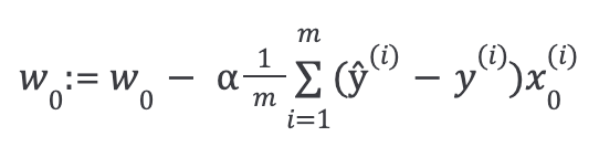
In order to minimize the error, we use the gradient descent algorithm. We keep updating the model parameters to move closer to the values that result in minimum cost.

Then repeat until convergence, with regularization: 

With some manipulation, the above equation can also be represented as:

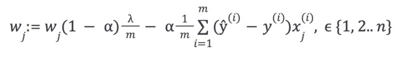
The first term in the above equation will always be less than one:

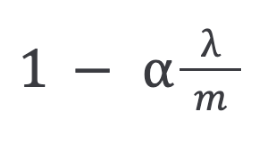
You can see it as reducing the value of the coefficient by some amount on every update.

Logistic Regression With Regularization

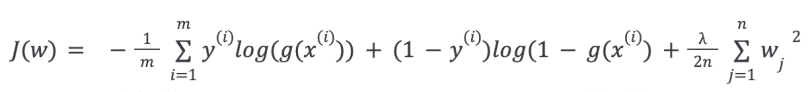
The cost function of the logistic regression with regularization is:

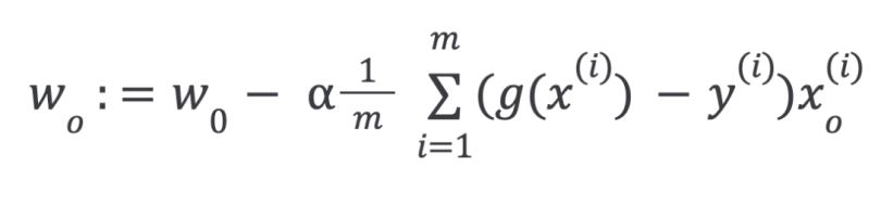
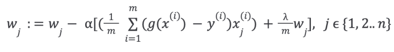
Then, repeat until convergence with regularization: 

L1 and L2 Regularization

The regularization term used in the previous equations is called L2, or ridge regularization.

The L2 penalty aims to minimize the squared magnitude of the weights.

There is another regularization called L1, or lasso:

The L1 penalty aims to minimize the absolute value of the weights.

Difference between L1 and L2

• L2 shrinks all the coefficients by the same proportions but eliminates none. 
• L1 can shrink some coefficients to zero, thus performing feature selection. 

Hyperparameters

Hyperparameters are higher-level parameters that describe structural information about a model that must be decided before fitting model parameters. Examples of hyperparameters we discussed so far include: Learning rate (alpha) and regularization (lambda).

Cross-Validation

The process to select the optimal values of hyperparameters is called model selection. if we reuse the same test data set over and over again during model selection, it will become part of our training data, and the model will be more likely to over fit.

The overall data set is divided into three categories:

1. Training data set.
2. Validation data set.
3. Test data set.

The training set is used to fit the different models, and the performance on the validation set is then used for the model selection. The advantage of keeping a test set that the model hasn’t seen before during the training and model selection steps is to avoid overfitting the model. The model is able to better generalize to unseen data.

In many applications, however, the supply of data for training and testing will be limited, and in order to build good models, we wish to use as much of the available data as possible for training. However, if the validation set is small, it will give a relatively noisy estimate of predictive performance. One solution to this dilemma is to use cross-validation.

More on Machine LearningUnderstanding Feature Importance in Machine Learning

7 Steps of Cross-Validation

These are the steps for selecting hyper-parameters using K-fold cross-validation:

1. Split your training data into K = 4 equal parts, or “folds.”
2. Choose a set of hyperparameters you wish to optimize.
3. Train your model with that set of hyperparameters on the first three folds.
4. Evaluate it on the fourth fold, or the hold-out fold.
5. Repeat steps (3) and (4) four times with the same set of hyperparameters, each time holding out a different fold.
6. Aggregate the performance across all four folds. This is your performance metric for the set of hyperparameters.
7. Repeat steps (2) to (6) for all sets of hyperparameters you wish to consider.

Cross-validation allows us to tune hyperparameters with only our training set. This allows us to keep the test set as a truly unseen data set for selecting the final model.

We’ve covered some of the key concepts in the field of machine learning, starting with the definition of machine learning and then covering different types of machine learning techniques. We discussed the theory behind the most common regression techniques (linear and logistic) alongside other key concepts of machine learning.