

Gradient descent is a popular optimization strategy that is used when training data models, can be combined with every algorithm and is easy to understand and implement. Everyone working with machine learning should understand its concept. We’ll walk through how the gradient descent algorithm works, what types of it are used today and its advantages and tradeoffs.
What Is Gradient Descent in Machine Learning?
Gradient Descent is an optimization algorithm for finding a local minimum of a differentiable function. Gradient descent in machine learning is simply used to find the values of a function's parameters (coefficients) that minimize a cost function as far as possible.
What Is Gradient Descent?
Gradient descent is an optimization algorithm that’s used when training a machine learning model. It’s based on a convex function and tweaks its parameters iteratively to minimize a given function to its local minimum.
You start by defining the initial parameter’s values and from there the gradient descent algorithm uses calculus to iteratively adjust the values so they minimize the given cost-function. To understand this concept fully, it’s important to know about gradients.
What Is a Gradient?
A gradient simply measures the change in all weights with regard to the change in error. You can also think of a gradient as the slope of a function. The higher the gradient, the steeper the slope and the faster a model can learn. But if the slope is zero, the model stops learning. In mathematical terms, a gradient is a partial derivative with respect to its inputs.
Imagine a blindfolded man who wants to climb to the top of a hill with the fewest steps possible. He might start climbing the hill by taking really big steps in the steepest direction. But as he comes closer to the top, his steps will get smaller and smaller to avoid overshooting it. Imagine the image below illustrates our hill from a top-down view and the red arrows are the steps of our climber. A gradient in this context is a vector that contains the direction of the steepest step the blindfolded man can take and how long that step should be.
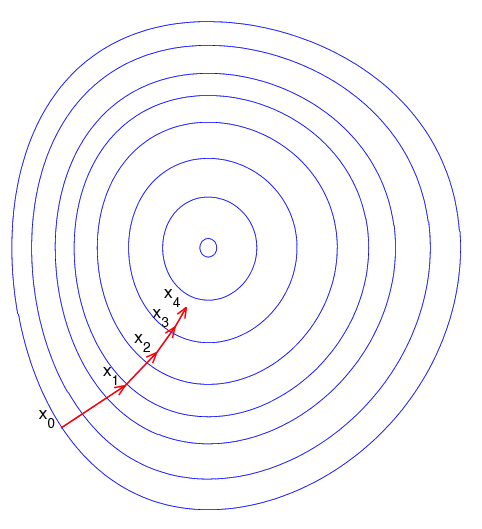
Note that the gradient ranging from X0 to X1 is much longer than the one reaching from X3 to X4. This is because the steepness/slope of the hill, which determines the length of the vector, is less. This perfectly represents the example of the hill because the hill is getting less steep the higher it’s climbed, so a reduced gradient goes along with a reduced slope and a reduced step size for the hill climber.
How Does Gradient Descent Work?
Instead of climbing up a hill, think of gradient descent as hiking down to the bottom of a valley. The equation below describes what the gradient descent algorithm does: b is the next position of our climber, while a represents his current position. The minus sign refers to the minimization part of the gradient descent algorithm. The gamma in the middle is a waiting factor and the gradient term ( Δf(a) ) is simply the direction of the steepest descent.
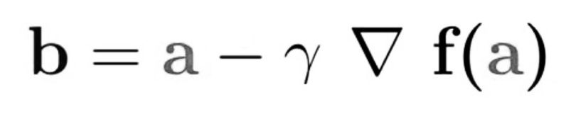
This formula basically tells us the next position we need to go, which is the direction of the steepest descent. Let’s look at another example to really drive the concept home.
Imagine you have a machine learning problem and want to train your algorithm with gradient descent to minimize your cost-function J(w, b) and reach its local minimum by tweaking its parameters (w and b). The image below shows the horizontal axes representing the parameters (w and b), while the cost function J(w, b) is represented on the vertical axes.
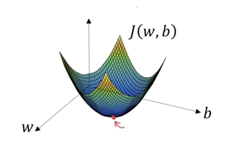
We want to find the values of w and b that correspond to the minimum of the cost function (marked with the red arrow). To start, we initialize w and b with some random numbers. Gradient descent then starts at that point (somewhere around the top of our illustration), and it takes one step after another in the steepest downside direction (i.e., from the top to the bottom of the illustration) until it reaches the point where the cost function is as small as possible.
Types of Gradient Descent
There are three popular types of gradient descent that mainly differ in the amount of data they use — batch, stochastic and mini-batch.
Batch Gradient Descent
Batch gradient descent, also called vanilla gradient descent, calculates the error for each example within the training dataset, but it only gets updated after all training examples have been evaluated. This process is like a cycle and called a training epoch.
An advantage of batch gradient descent is its computational efficiency: it produces a stable error gradient and a stable convergence. But the stable error gradient can sometimes result in a state of convergence that isn’t the best the model can achieve. It also requires the entire training dataset to be in memory and available to the algorithm.
Stochastic Gradient Descent
By contrast, stochastic gradient descent (SGD) does this for each training example within the dataset, meaning it updates the parameters for each training example one by one. Depending on the problem, this can make SGD faster than batch gradient descent. One advantage is that frequent updates allow us to have a pretty detailed rate of improvement.
The frequent updates, however, are more computationally expensive than the batch gradient descent approach. Additionally, the frequency of those updates can result in noisy gradients, which may cause the error rate to jump around instead of slowly decreasing.
Mini-Batch Gradient Descent
Mini-batch gradient descent is the go-to method since it’s a combination of the concepts of SGD and batch gradient descent. It simply splits the training dataset into small batches and performs an update for each of those batches. This creates a balance between the robustness of stochastic gradient descent and the efficiency of batch gradient descent.
Common mini-batch sizes range between 50 and 256, but like any other machine learning technique, there is no clear rule because it varies for different applications. This is the go-to algorithm when training a neural network, and it’s the most common type of gradient descent within deep learning.
Gradient Descent Learning Rate
How big the steps gradient descent takes in the direction of the local minimum is determined by the learning rate, which figures out how fast or slow we will move towards the optimal weights.
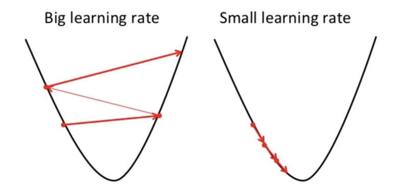
For the gradient descent algorithm to reach the local minimum, we must set the learning rate to an appropriate value, which is neither too low nor too high. This is important because if the steps it takes are too big, it may not reach the local minimum because it bounces back and forth between the convex function of gradient descent (see left image below). If we set the learning rate to a very small value, gradient descent will eventually reach the local minimum but that may take a while (see the right image).
The learning rate should never be too high or too low for this reason. You can check if your learning rate is doing well by plotting it on a graph.
How to Solve Gradient Descent Challenges
To make sure the gradient descent algorithm runs properly, plot the cost function as the optimization runs. Put the number of iterations on the x-axis and the value of the cost function on the y-axis. This helps you see the value of your cost function after each iteration of gradient descent, and provides a way to easily spot how appropriate your learning rate is. Try different values for it and plot them all together. The left image below shows such a plot, while the image on the right illustrates the difference between good and bad learning rates.
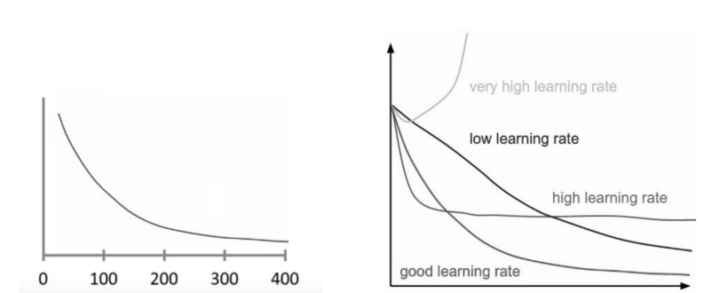
If the gradient descent algorithm is working properly, the cost function should decrease after every iteration.
When gradient descent can’t decrease the cost function anymore and remains more or less on the same level, it has converged. The number of iterations gradient descent needs to converge can sometimes vary a lot. It can take 50 iterations, 60,000 or maybe even 3 million, making the number of iterations to convergence hard to estimate in advance.
There are some algorithms that can automatically tell you if gradient descent has converged, but you must define a threshold for the convergence beforehand, which is also pretty hard to estimate. For this reason, simple plots are the preferred convergence test.
Another advantage of monitoring gradient descent via plots is it allows us to easily spot if it doesn’t work properly, for example if the cost function is increasing. Most of the time the reason for an increasing cost-function when using gradient descent is a learning rate that’s too high.
If the plot shows the learning curve going up and down without really reaching a lower point, try decreasing the learning rate. Also, when starting out with gradient descent on a given problem, simply try 0.001, 0.003, 0.01, 0.03, 0.1, 0.3, 1, etc., as the learning rates and look at which one performs the best.
Frequently Asked Questions
What is gradient descent?
Gradient descent is an optimization algorithm often used to train machine learning models by locating the minimum values within a cost function. Through this process, gradient descent minimizes the cost function and reduces the margin between predicted and actual results, improving a machine learning model’s accuracy over time.
What are the three types of gradient descent?
The three types of gradient descent are batch gradient descent, stochastic gradient descent and mini-batch gradient descent.


