Probability distributions are one of the most used mathematical concepts used in various real-life applications. From weather prediction to the stock market to machine learning applications, different probability distributions are the basic building blocks of all these applications and more. If you want to break into the world of data science, knowing the basics of probability theory in general and the most common probability distribution, in particular, is must-have knowledge.
4 Common Probability Distributions for Data Scientists
- Normal (Gaussian) distribution
- Binomial distribution
- Uniform distribution
- Poisson distribution
Probability Theory Basics
Probability theory (PT) is a well-established branch of mathematics that deals with the uncertainties in our lives. In PT, an experiment is any process that could be repeated and have a set of well-known different outcomes.
For example: rolling dice. We can repeat the experiment and the dice can fall on one of six constant faces. Each experiment has a sample space that represents all the possible outcomes of that experiment. In the case of rolling a die, our sample space will be {1,2,3,4,5,6}.
Finally, every try of the experiment is called an event.
Theoretical vs. Experimental Probability
Theoretically, we can calculate the probability of every outcome using the following formula:

If we consider rolling dice, the probability of the dice landing on any of the six sides is 0.166. If I want to know the probability of the dice landing on an even number, then it will be 0.5, because, in this case, the desired outcomes are {2,4,6} out of the full sample space {1,2,3,4,5,6}.
The sum of the probabilities of all possible outcomes should always equal one.
Externally, the probability of any outcome can be a little different from the theoretical one; however, if we repeat the experiment enough times, then the experimental probability will come close to the theoretical one.
We can write simple Python code to prove the difference between theoretical and experimental probabilities.
from random import randint
from collections import Counter
#A function to genrate random experiments
def gen(x):
    expResults = []
    for i in range(x):
        expResults.append(randint(1,6))
    return expResults
#An experiment with 100 events
event1 = dict(Counter(gen(100)))
for k,v in event1.items():
  print("probability of", k, "is",v/100)
print("------------------------------")
#An experiment with 1000 events
event2 = dict(Counter(gen(1000)))
for k,v in event2.items():
  print("probability of", k, "is",v/1000)
The results of running this code will be close to:
probability of 1 is 0.16
probability of 2 is 0.15
probability of 3 is 0.18
probability of 4 is 0.12
probability of 5 is 0.18
probability of 6 is 0.21
— — — — — — — — — — — — — — —
probability of 1 is 0.16
probability of 2 is 0.179
probability of 3 is 0.168
probability of 4 is 0.162
probability of 5 is 0.154
probability of 6 is 0.177
As you can see, the more trials we have, the closer we get to the theoretical probability value.
Random Variables
Random variables (RV) have variables determined by the outcome of a random experiment. Going back to our dice, if we define a random variable X as the probability of any outcome, then P(X=5) = 0.166.
There are two types of random variables:
-
Discrete random variables: Random variables that can take a countable number of distinct values (like the possible outcomes of rolling dice).
-
Continuous random variables: Random variables that can take an infinite number of values in an interval (such as the temperature of Tokyo on any August day).
Probability Distributions
Probability distributions are simply a collection of data (or scores) of a particular random variable. Usually, these collections of data are arranged in some order and can be presented graphically. Whenever we start a new DS project, we typically obtain a data set; this data set represents a sample from a population, which is a larger data set. Using this sample, we can try and find distinctive patterns in the data that help us make predictions about our main inquiry.
For example, if we want to buy shares from the stock market, we can take a sample data set from the last five to 10 years of a specific company, analyze that sample and predict the future price of shares.
Distribution Characteristics
Data distributions have different shapes; the data set used to draw the distribution defines the distribution’s shape. We can describe each distribution using three characteristics: the mean, the variance and the standard deviation. These characteristics can tell us different things about the distribution’s shape and behavior.
Mean
The mean (μ) is simply the average of a data set. For example, if we have a set of discrete data {4,7,6,3,1}, the mean is 4.2.
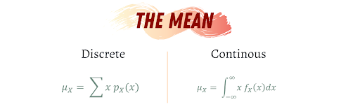
The mean (μ) is simply the average of a data set. For example, if we have a set of discrete data {4,7,6,3,1}, the mean is 4.2.
Variance
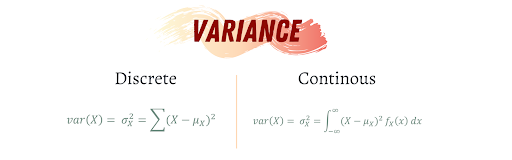
The variance (var(X)) is the average of the squared differences from the mean. For example, if we have the same data set from before {4,7,6,3,1}, then the variance will be 5.7.
Standard Deviation
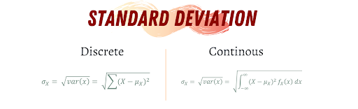
The standard deviation (σ) is a measure of how spread out the numbers are in a data set. So, a small standard deviation indicates that the values are closer to each other, while a large standard deviation indicates the data set values are spread out.
Properties of Mean, Variance & Standard Deviation
-
If all the values in a data set are the same, the standard deviation will equal zero.
-
If the values of a data set have been shifted (add or subtract a constant from all values), the mean will increase or decrease the amount of the shift while the variance will remain unchanged. For example, if we shift a data set by 10, then the mean will increase by 10.
-
If the values of a data set have been scaled (multiplied by a constant), the mean will be scaled by the same factor, while the variance will be scaled by the absolute value of the factor. For example, if we scale a data set by 10, then the mean will be scaled by 10. However, if we scale it by -10, the mean will scale by -10 while the variance will scale by 10 in both cases.
The 4 Most Common Distributions
There are many different probability distributions out there; some of them are more common than others. Let’s look at the four most commonly used distributions in data science.
1. Normal Distribution
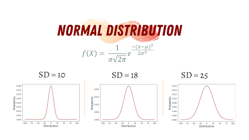
Gaussian distribution (normal distribution) is famous for its bell-like shape, and it’s one of the most commonly used distributions in data science. Many real-life phenomena follow normal distribution, such as peoples’ height, the size of things produced by machines, errors in measurements, blood pressure and grades on a test.
Normal Distribution Characteristics
The key characteristics of the normal distribution are:
-
The curve is symmetric at the center, which means it can be divided into two even sections around the mean.
-
Because the normal distribution is a probability distribution, the area under the distribution curve is equal to one.
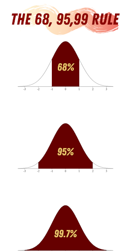
When dealing with the normal distribution, there’s one important thing to keep in mind: the 68, 95, 99 rule. This rule states that 68% of the data in a normal distribution is between -σ and σ, 95% will be between -2σ and 2σ, and 99.7% of the data will be between -3σ and 3σ.
Various machine learning models work on data sets that follow a normal distribution, such as Gaussian Naive Bayes classifier, linear and quadratic discriminant analysis, and least square-based regression. Moreover, we can transform non-normal distributed data sets into normally distributed ones, using some mathematical transformation algorithms such as taking the square root, inverse or natural log of the original data. Here’s how to generate normal distributions using Python.
#Import Essential Libraries
import numpy as np
import matplotlib.pyplot as plt
import scipy.stats as stat
#Normal Distribution
n = np.arange(-100, 100)
mean = 0
sd = 15
normalDist = stat.norm.pdf(n, mean, sd)
plt.plot(n, normalDist, color="#8d0801")
plt.xlabel('Distribution', fontsize=15 ,color="#001427")
plt.ylabel('Probability', fontsize=15, color="#001427")
plt.title("Normal Distribution", color="#001427")
Exponential Distribution
The exponential distribution is not a generalization of the normal distribution. Therefore, it’s also known as the generalized normal distribution. Nevertheless, the exponential distribution has two more factors λ, which represent the positive scale parameter (squeezes or stretches a distribution) and κ, which represents the positive shape parameter (alters the shape of the distribution). Additionally, The exponential distribution doesn’t allow for asymmetrical data, so it's more of a skewed normal distribution.
2. Binomial Distribution
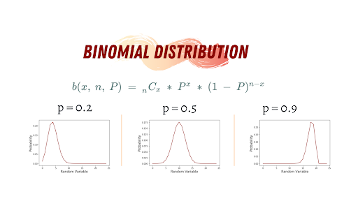
A binomial experiment is a statistical experiment, where a binomial random variable is the number of successes (x) in repeated trials of a binomial experiment (n). The probability distribution of a binomial random variable is called a binomial distribution.
Conditions of the Binomial Distribution
-
It is made of independent trials.
-
Each trial can be classified as either success or failure, where the probability of success is p while the probability of failure is 1-p.
-
It has a fixed number of trials (n).
-
The probability of success in each trial is constant.
Some examples of binomial distributions in daily life:
-
If a brand new drug or vaccine is introduced to cure a disease, it either cures the disease (success) or it doesn’t (failure).
-
If you buy a lottery ticket, you either win money or you don’t.
Basically, anything you can think about which has two possible outcomes can be represented by a binomial distribution.
Another way to think about binomial distribution is that they’re the discrete version of limited normal distribution. The normal distribution is the result of many continuous trials of binomial distribution. Here’s how to generate a binomial distribution using Python.
#Import Essential Libraries
import numpy as np
import matplotlib.pyplot as plt
import scipy.stats as stat
#Generate the Binomial Distribution
x = np.arange(0, 25)
noOfTrials = 20 #Number of trials
prob = 0.9 #probability of success
binom = stat.binom.pmf(x, noOfTrials, prob)
plt.plot(x, binom, color="#8d0801")
plt.xlabel('Random Variable', fontsize=15)
plt.ylabel('Probability', fontsize=15)
Bernoulli Distribution
Bernoulli distribution is a particular case of the binomial distribution. It is a binomial distribution with only one trial.
3. Uniform Distribution
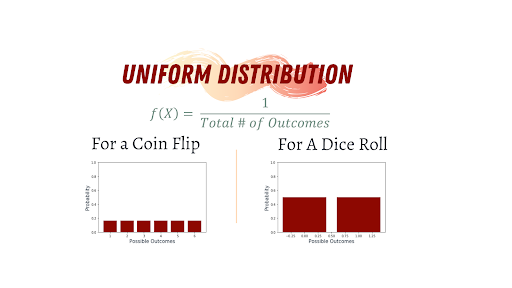
A uniform distribution, also called a rectangular distribution, is a probability distribution that has a constant probability, such as flipping a coin or rolling dice. This distribution has two types. The most common type in elementary statistics is the continuous uniform distribution (which forms the shape of a rectangle). The second type is the discrete uniform distribution. Here’s how to generate a uniform distribution in Python.
#Import Essential Libraries
import numpy as np
import matplotlib.pyplot as plt
#Generating Uniform Distribution for a Dice Roll
probs = np.full(6, 1/6)
faces = [1,2,3,4,5,6]
plt.bar(faces, probs, color="#8d0801")
plt.ylabel('Probability', fontsize=15 ,color="#001427")
plt.xlabel('Possible Outcomes', fontsize=15 ,color="#001427")
axes = plt.gca()
axes.set_ylim([0,1])
4. Poisson Distribution
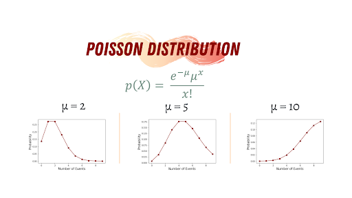
The Poisson random variable satisfies the following conditions:
-
The number of successes in two disjointed time intervals is independent, and the average of successes is μ.
-
The probability of success during a small time interval is proportional to the entire length of the time interval.
Poisson distribution can be found in many phenomena, such as congenital disabilities and genetic mutations, car accidents, meteor showers, traffic flow and the number of typing errors on a page. Also, business professionals employ Poisson distributions to create forecasts about the number of shoppers or sales on certain days or seasons of the year. In business, overstocking will sometimes mean losses if the products aren’t sold. Similarly, understocking causes the loss of business opportunities because you are not able to maximize your sales. By using this distribution, business owners can predict when the demand is high so they can buy more stock. Here’s the code to generate a poisson distribution in Python.
#Importing Essential Libraries
import numpy as np
import matplotlib.pyplot as plt
import scipy.stats as stat
#Genrating the Poisson Distribution
n = np.arange(0, 10)
mu = 2 #average number of events
poisson = stat.poisson.pmf(n, lamda)
plt.plot(n, poisson, '-s', label="Mu = {:f}".format(mu), color="#8d0801")
plt.xlabel('# of Events', fontsize=15)
plt.ylabel('Probability', fontsize=15)
There are many more distributions out there to learn. However, knowing these four will get you started as you launch your data science career.
Frequently Asked Questions
What is the difference between theoretical and experimental probability?
Theoretical probability is calculated based on known possible outcomes, while experimental probability is based on the results of actual repeated trials. With enough trials, experimental results tend to approach theoretical values.
What are random variables and how are they used in probability distributions?
Random variables represent outcomes of a random experiment. They can be discrete (countable outcomes, like dice rolls) or continuous (infinite outcomes within a range, like temperature).
What is the 68-95-99.7 rule in a normal distribution?
It states that in a normal distribution, approximately 68 percent of data falls within one standard deviation of the mean, 95 percent within two and 99.7 percent within three.