A Step-by-Step Explanation of Stochastic Policy Gradient Algorithms

As you might remember from my previous tutorials on deep Q-learning and deep (double) Q-learning, we’re able to control an AI in discrete action spaces, where the possible actions may be as simple as going left or right, up or down. Despite these simple possibilities the AI agents are still able to accomplish astonishing tasks such as playing Atari with a super-human performance or beating the world’s best human player in the board game Go.

However many real-world applications of reinforcement learning (such as training robots or self-driving cars) require an agent to select optimal actions from continuous spaces. Let’s dive into the concept of continuous action space with an example.

When you’re driving your car and you turn the steering wheel, you can control to what degree you turn it. This leads to a continuous action space (e.g., for each positive real number x in some range, “turn the wheel x degrees to the right”). Or consider how hard you press the gas pedal down. That’s a continuous input, as well.

Remember: Continuous action space means there is (theoretically) an infinite amount of possible actions.

In fact, most actions that we’ll ever encounter in real life are from the continuous action space. That is why it’s so important to understand how we can train an AI that selects an action if there are an infinite amount of possibilities.

This is where stochastic policy gradient algorithms are beneficial.

What Do Stochastic Policy Gradient Algorithms Do?

Update the parameters θ of the actor π towards the gradient of the performance J(θ)
Update parameters w of the critic, with regular temporal difference learning algorithms

How can you practice stochastic policy gradients?

This example of OpenAI’s Gym MountainCarContinuous problem was solved with stochastic policy gradients, presented here. The well-documented source code can be found in my GitHub repository. I have chosen MountainCarContinuous as an example because the training time for this problem is very low and you can reproduce it yourself quickly. If you want to practice after reading this article, clone the repository and execute src/policy gradients/stochastic/ stochastic_pg.py to start the algorithm.

Hold Up. Start Over.How AI Teach Themselves Through Deep Reinforcement Learning

Stochastic Policy

In part one of this series, I introduced the AI agent as a neural network that interacts with the environment (computer game, chessboard, etc.) by observing its states s (screen pixels, board-configuration, etc.) and taking actions a, based on the current observable state s.

For each action a in a state s the AI agent receives a reward. The amount of the reward tells the agent the quality of his action in this particular state with regards to solving the given objective (e.g., learning how to walk or winning a game). The actions in any given state are determined by the policy π.

Previously, I introduced the policy as the strategy of the AI that determines his movement from one state s to the next state s’, across the whole sequence of all possible states s_1, ..., s_n in the environment.

In part two of this series, I demonstrated how the agent follows the policy π, which tells it to take actions in a state s which correspond to the highest action-value Q(s,a). The action-value function is the expected return (i.e., the sum of reward across all states) we obtain by starting in state s, taking action a and then following the policy π.

In the case of stochastic policies, the basic idea is to represent the policy by a parametric probability distribution:

The distribution stochastically selects action a in state s according to a parameter vector θ. We can look at the Gaussian distribution as an example of the policy as a probability distribution, where we stochastically pick an action a, as a sample from this distribution (figure 1). This yields action a as a continuous variable.

Note: In contrast to deep Q-learning, the policy π is now a direct mapping/function from a state s to an action a.

More From Artem OppermannA Deep Dive Into Deep Q-Learning

One-Step Process

But how do we determine if the current policy π is a good one? To do this we must define a performance function for π, which we call J(θ).

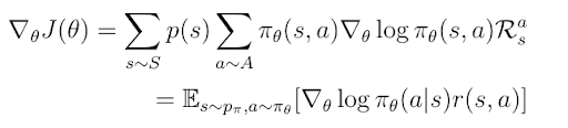
Let’s discuss a simple case, where we want to measure the quality/performance of π for only one step of the agent (from the state s to the next state s’). In this case, we can define the quality function as follows:

The second line in the equation is nothing other than the execution of the expectation operator E on the expected action-value r(s,a) for the action a in state s. s is selected from the environment, while a is selected according to the policy π. R_a_s is the reward for the action a in state s.

Please note: r(s,a) means the same as Q(s,a) or q(s,a) but for a one-step process.

We must consider that in deep reinforcement learning the environment is stochastic, meaning taking an action does not guarantee that the agent will end up in the state it intends to. It’s up to the environment to decide to a certain degree where the agent will actually end up. Because the action-value r(s,a) depends also on the next state s’ (see equation 17 in part one of this series) we must average the reward R_a_s overall transitional probabilities p(s):=p(s→s’) from state s to the next state s’. Furthermore, because R_a_s also depends on the action, we must average the reward over all possible π(a,s).

Back to BasicsArtificial Intelligence vs. Machine Learning vs. Deep Learning

Stochastic Policy Gradient Theorem

Policy gradient algorithms typically proceed by sampling this stochastic policy and adjusting the policy parameters in the direction of greater cumulative reward.

Now that we’ve defined the performance of the policy π, we can go further and discuss how the agent can learn the optimal policy. Since π(θ) depends on some parameters θ (which are, in most cases, the weights and biases of a neural network) we must find optimal θ which maximize the performance.

The basic idea behind the policy gradient method is to adjust these parameters θ of the policy in the direction of the performance gradient.

If we calculate the gradient of J(θ) we obtain the following expression:

Because we want to find θ, which maximizes the performance, we must update θ doing gradient ascent — in contrast to gradient descent where we want to find parameters which minimize a predefined loss function.

Policy Gradient Methods from DeepMind

Multi-Step Process

Now that we know how to improve the policy for a one-step process, we can continue with the case wherein we consider the process of the AI agent’s movement across the whole sequence of states.

Actually, this case is not that difficult if we keep in mind that the sum of (discounted) rewards we would receive during this process of movements from one state to another following a policy π, is the exact definition of the action-value function Q(s,a). This yields the following definition of the policy gradient for the multi-step-process, where the single expected reward r(s,a) is exchanged with the expected cumulative return (sum of rewards) Q(s,a).

Deep Learning Nuts and Bolts5 Deep Learning Activation Functions You Need to Know

Actor-Critic Algorithms

We call the algorithms that use the update rule actor-critic algorithms (see equation 4). The policy π(a|s) is called the actor because the actor determines the action that must be taken in a state s. Meanwhile, the critic Q(s,a), serves the purpose of criticizing the actor’s action by giving it a quality/value.

As you can see, the gradient of J(θ) scales with this quality-value. A high quality/value suggests the action a in state s was in fact a good choice, and the update of θ in the direction of performance can be increased. The opposite applies to the small quality/value.

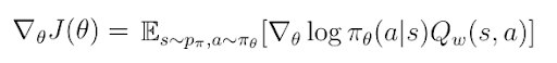
In reality, we cannot know Q(s,a) in advance so we must approximate it by a function Q_w(s,a) which depends on parameters w. In general Q_w(s,a) can be estimated by a neural network.

That yields a new definition for the performance gradient:

In summary, a stochastic policy gradient algorithm tries to:

Update the parameters θ of the actor π towards the gradient of the performance J(θ)
Update parameters w of the critic, with regular temporal difference learning algorithms, which I introduced in deep Q-learning.

The whole actor-critic algorithm can be expressed by the following pseudocode:

The crucial part of the algorithm happens in the for-loop which represents the lifetime of the AI-agent. Let’s discuss each step in more depth:

Receive a reward R from the environment by taking action a in state s, and observe the new state s’.
Given this new state s’ sample an action a’ stochastically from the distribution π.
Calculate the temporal difference target delta using old s, a and new s’, a’.
Update the parameters w according to the temporal difference learning update rule. (Better alternative: Update w by minimizing the distance between r+ γQ(s’,a’) and Q(s,a) with regular gradient descent algorithms.)
Update the parameters θ of the policy by performing a gradient ascent step towards the gradient of the performance J(θ).
Set new state s’ as old state s, and new action a’ as old action a.
Begin the loop from the beginning if the process has not been terminated

Reducing Variance

The vanilla implementation of the actor-critic algorithm is known for having a high variance. One possibility to reduce this variance is to subtract from the action-value Q(s,a) the state-value V(s) (equation 7). I defined the state value in Markov decision processes as the expected total reward the AI agent will receive if it starts its progress in the state s, without considering the actions.

This new term is defined as the advantage and can be inserted into the gradient of the performance. Using the advantage has shown promising results in reducing the variance of the algorithm.

On the other side with the advantage, we introduce the problem of the requirement to have a third function approximator like a neural network to estimate V(s). However, we can demonstrate that the expected temporal difference error of V(s) (equation 9) is nothing other than the advantage.

We can demonstrate this by using one definition of Q(s,a), which is the expected value of r+γV(s’). By subtracting the remaining term V(s) we obtain the previous definition of the advantage A (equation 10).