Machine learning is the science (and art) of programming computers so they can learn from data.
[Machine learning is the] field of study that gives computers the ability to learn without being explicitly programmed. — Arthur Samuel, 1959
A better definition:
A computer program is said to learn from experience E with respect to some task T and some performance measure P, if its performance on T, as measured by P, improves with experience E. — Tom Mitchell, 1997
For example, your spam filter is a machine learning program that can learn to flag spam after being given examples of spam emails that are flagged by users, and examples of regular non-spam (also called “ham”) emails. The examples the system uses to learn are called the training set. In this case, the task (T) is to flag spam for new emails, the experience (E) is the training data, and the performance measure (P) needs to be defined. For example, you can use the ratio of correctly classified emails as P. This particular performance measure is called accuracy and it is often used in classification tasks as it is a supervised learning approach.
Supervised Machine Learning Classification
In supervised machine learning, algorithms learn from labeled data. After understanding the data, the algorithm determines which label should be given to new data by associating patterns to the unlabeled new data.
Supervised learning can be divided into two categories: classification and regression.
What Is Classification?
Classification predicts the category the data belongs to. Some examples of classification include spam detection, churn prediction, sentiment analysis, dog breed detection and so on.
What Is Regression?
Regression predicts a numerical value based on previously observed data. Some examples of regression include house price prediction, stock price prediction, height-weight prediction and so on.
5 Types of Classification Algorithms for Machine Learning
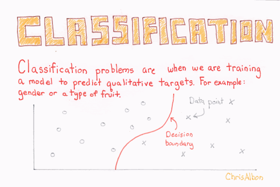
Classification is a technique for determining which class the dependent belongs to based on one or more independent variables.
What Is a Classifier?
Classification is used for predicting discrete responses.
1. Logistic Regression
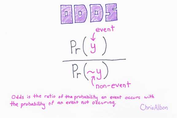
Logistic regression is kind of like linear regression, but is used when the dependent variable is not a number but something else (e.g., a “yes/no” response). It’s called regression but performs classification based on the regression and it classifies the dependent variable into either of the classes.

Logistic regression is used for prediction of output which is binary, as stated above. For example, if a credit card company builds a model to decide whether or not to issue a credit card to a customer, it will model for whether the customer is going to “default” or “not default” on their card.

Firstly, linear regression is performed on the relationship between variables to get the model. The threshold for the classification line is assumed to be at 0.5.

Logistic function is applied to the regression to get the probabilities of it belonging in either class.
It gives the log of the probability of the event occurring to the log of the probability of it not occurring. In the end, it classifies the variable based on the higher probability of either class.
2. K-Nearest Neighbors (K-NN)
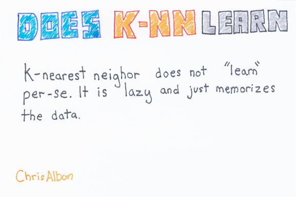
K-NN algorithm is one of the simplest classification algorithms and it is used to identify the data points that are separated into several classes to predict the classification of a new sample point. K-NN is a non-parametric, lazy learning algorithm. It classifies new cases based on a similarity measure (i.e., distance functions).
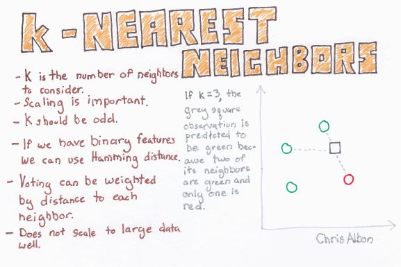



K-NN works well with a small number of input variables (p), but struggles when the number of inputs is very large.
3. Support Vector Machine (SVM)
Support vector is used for both regression and classification. It is based on the concept of decision planes that define decision boundaries. A decision plane (hyperplane) is one that separates between a set of objects having different class memberships.

It performs classification by finding the hyperplane that maximizes the margin between the two classes with the help of support vectors.

The learning of the hyperplane in SVM is done by transforming the problem using some linear algebra (i.e., the example above is a linear kernel which has a linear separability between each variable).
For higher dimensional data, other kernels are used as points and cannot be classified easily. They are specified in the next section.
Kernel SVM
Kernel SVM takes in a kernel function in the SVM algorithm and transforms it into the required form that maps data on a higher dimension which is separable.
Types of kernel functions:

- Linear SVM is the one we discussed earlier.
- In polynomial kernel, the degree of the polynomial should be specified. It allows for curved lines in the input space.
- In the radial basis function (RBF) kernel, it is used for non-linearly separable variables. For distance, metric squared Euclidean distance is used. Using a typical value of the parameter can lead to overfitting our data. It is used by default in sklearn.
- Sigmoid kernel, similar to logistic regression is used for binary classification.
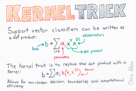
Kernel trick uses the kernel function to transform data into a higher dimensional feature space and makes it possible to perform the linear separation for classification.
Radial Basis Function (RBF) Kernel
The RBF kernel SVM decision region is actually also a linear decision region. What RBF kernel SVM actually does is create non-linear combinations of features to uplift the samples onto a higher-dimensional feature space where a linear decision boundary can be used to separate classes.
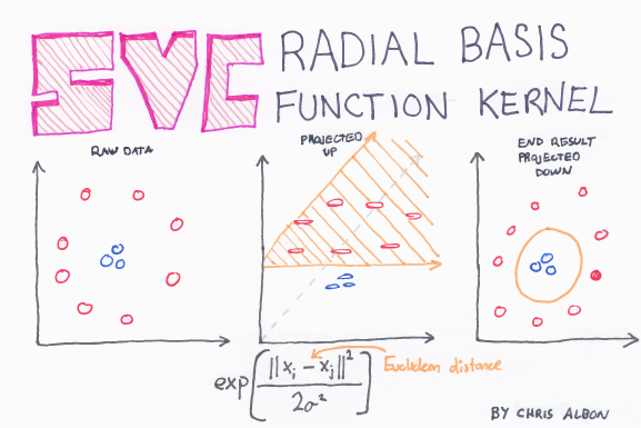
So, the rule of thumb is: use linear SVMs for linear problems, and nonlinear kernels such as the RBF kernel for non-linear problems.
4. Naive Bayes
The naive Bayes classifier is based on Bayes’ theorem with the independence assumptions between predictors (i.e., it assumes the presence of a feature in a class is unrelated to any other feature). Even if these features depend on each other, or upon the existence of the other features, all of these properties independently. Thus, the name naive Bayes.

Based on naive Bayes, Gaussian naive Bayes is used for classification based on the binomial (normal) distribution of data.

- P(class|data) is the posterior probability of class(target) given predictor(attribute). The probability of a data point having either class, given the data point. This is the value that we are looking to calculate.
- P(class) is the prior probability of class.
- P(data|class) is the likelihood, which is the probability of predictor given class.
- P(data) is the prior probability of predictor or marginal likelihood.
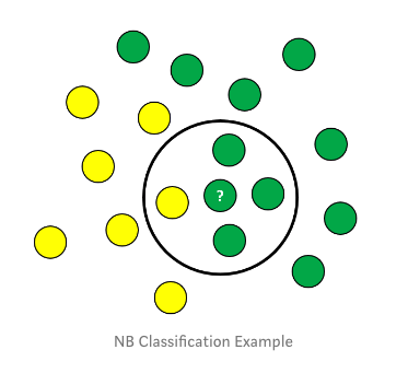
Naive Bayes Steps
1. Calculate Prior Probability
P(class) = Number of data points in the class/Total no. of observations
P(yellow) = 10/17
P(green) = 7/17
2. Calculate Marginal Likelihood
P(data) = Number of data points similar to observation/Total no. of observations
P(?) = 4/17
The value is present in checking both the probabilities.
3. Calculate Likelihood
P(data/class) = Number of similar observations to the class/Total no. of points in the class.
P(?/yellow) = 1/7
P(?/green) = 3/10
4. Posterior Probability for Each Class
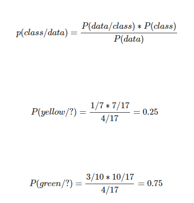
5. Classification
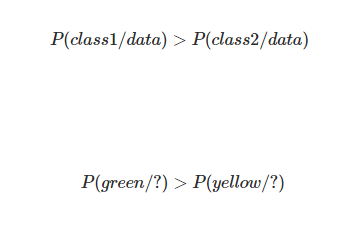
The higher probability, the class belongs to that category as from above 75% probability the point belongs to class green.
Multinomial, Bernoulli naive Bayes are the other models used in calculating probabilities. Thus, a naive Bayes model is easy to build, with no complicated iterative parameter estimation, which makes it particularly useful for very large datasets.
5. Decision Tree Classification
Decision tree builds classification or regression models in the form of a tree structure. It breaks down a dataset into smaller and smaller subsets while at the same time an associated decision tree is incrementally developed. The final result is a tree with decision nodes and leaf nodes. It follows Iterative Dichotomiser 3 (ID3) algorithm structure for determining the split.
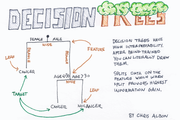
Entropy and information gain are used to construct a decision tree.
Entropy
Entropy is the degree or amount of uncertainty in the randomness of elements. In other words, it is a measure of impurity.
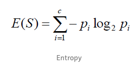
Intuitively, it tells us about the predictability of a certain event. Entropy calculates the homogeneity of a sample. If the sample is completely homogeneous the entropy is zero, and if the sample is equally divided it has an entropy of one.
Information Gain
Information gain measures the relative change in entropy with respect to the independent attribute. It tries to estimate the information contained by each attribute. Constructing a decision tree is all about finding the attribute that returns the highest information gain (i.e., the most homogeneous branches).

Where Gain(T, X) is the information gain by applying feature X. Entropy(T) is the entropy of the entire set, while the second term calculates the entropy after applying the feature X.
Information gain ranks attributes for filtering at a given node in the tree. The ranking is based on the highest information gain entropy in each split.
The disadvantage of a decision tree model is overfitting, as it tries to fit the model by going deeper in the training set and thereby reducing test accuracy.

Overfitting in decision trees can be minimized by pruning nodes.
Ensemble Methods for Classification
An ensemble model is a team of models. Technically, ensemble models comprise several supervised learning models that are individually trained and the results merged in various ways to achieve the final prediction. This result has higher predictive power than the results of any of its constituting learning algorithms independently.

1. Random Forest Classification
Random forest classifier is an ensemble algorithm based on bagging i.e bootstrap aggregation. Ensemble methods combines more than one algorithm of the same or different kind for classifying objects (i.e., an ensemble of SVM, naive Bayes or decision trees, for example.)

The general idea is that a combination of learning models increases the overall result selected.

Deep decision trees may suffer from overfitting, but random forests prevent overfitting by creating trees on random subsets. The main reason is that it takes the average of all the predictions, which cancels out the biases.
Random forest adds additional randomness to the model while growing the trees. Instead of searching for the most important feature while splitting a node, it searches for the best feature among a random subset of features. This results in a wide diversity that generally results in a better model.
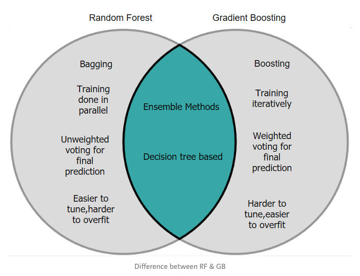
2. Gradient Boosting Classification
Gradient boosting classifier is a boosting ensemble method. Boosting is a way to combine (ensemble) weak learners, primarily to reduce prediction bias. Instead of creating a pool of predictors, as in bagging, boosting produces a cascade of them, where each output is the input for the following learner. Typically, in a bagging algorithm trees are grown in parallel to get the average prediction across all trees, where each tree is built on a sample of original data. Gradient boosting, on the other hand, takes a sequential approach to obtaining predictions instead of parallelizing the tree building process. In gradient boosting, each decision tree predicts the error of the previous decision tree — thereby boosting (improving) the error (gradient).

Working of Gradient Boosting
- Initialize predictions with a simple decision tree.
- Calculate residual (actual-prediction) value.
- Build another shallow decision tree that predicts residual based on all the independent values.
- Update the original prediction with the new prediction multiplied by learning rate.
- Repeat steps two through four for a certain number of iterations (the number of iterations will be the number of trees).
Check out this post: Gradient Boosting From Scratch
Metrics to Measure Classification Model Performance
1. Confusion Matrix
A confusion matrix is a table that is often used to describe the performance of a classification model on a set of test data for which the true values are known. It is a table with four different combinations of predicted and actual values in the case for a binary classifier.

The confusion matrix for a multi-class classification problem can help you determine mistake patterns.
For a binary classifier:
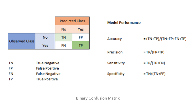
A true positive is an outcome where the model correctly predicts the positive class. Similarly, a true negative is an outcome where the model correctly predicts the negative class.
False Positive and False Negative
The terms false positive and false negative are used in determining how well the model is predicting with respect to classification. A false positive is an outcome where the model incorrectly predicts the positive class. And a false negative is an outcome where the model incorrectly predicts the negative class. The more values in main diagonal, the better the model, whereas the other diagonal gives the worst result for classification.
False Positive
False positive (type I error) — when you reject a true null hypothesis.
This is an example in which the model mistakenly predicted the positive class. For example, the model inferred that a particular email message was spam (the positive class), but that email message was actually not spam. It’s like a warning sign that the mistake should be rectified as it’s not much of a serious concern compared to false negative.

False Negative
False negative (type II error) — when you accept a false null hypothesis.
This is an example in which the model mistakenly predicted the negative class. For example, the model inferred that a particular email message was not spam (the negative class), but that email message actually was spam. It’s like a danger sign that the mistake should be rectified early as it’s more serious than a false positive.
Accuracy, Precision, Recall and F-1 Score
From the confusion matrix, we can infer accuracy, precision, recall and F-1 score.
Accuracy
Accuracy is the fraction of predictions our model got right.

Accuracy can also be written as

Accuracy alone doesn’t tell the full story when working with a class-imbalanced data set, where there is a significant disparity between the number of positive and negative labels. Precision and recall are better metrics for evaluating class-imbalanced problems.
Precision
Out of all the classes, precision is how much we predicted correctly.

Precision should be as high as possible.
Recall
Out of all the positive classes, recall is how much we predicted correctly. It is also called sensitivity or true positive rate (TPR).

Recall should be as high as possible.
F-1 Score
It is often convenient to combine precision and recall into a single metric called the F-1 score, particularly if you need a simple way to compare two classifiers. The F-1 score is the harmonic mean of precision and recall.
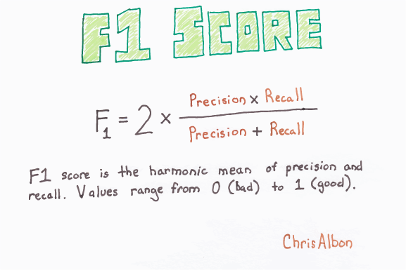
The regular mean treats all values equally, while the harmonic mean gives much more weight to low values thereby punishing the extreme values more. As a result, the classifier will only get a high F-1 score if both recall and precision are high.
2. Receiver Operator Curve (ROC) and Area Under the Curve (AUC)
ROC curve is an important classification evaluation metric. It tells us how well the model has accurately predicted. The ROC curve shows the sensitivity of the classifier by plotting the rate of true positives to the rate of false positives. If the classifier is outstanding, the true positive rate will increase, and the area under the curve will be close to one. If the classifier is similar to random guessing, the true positive rate will increase linearly with the false positive rate. The better the AUC measure, the better the model.

3. Cumulative Accuracy Profile Curve
The CAP of a model represents the cumulative number of positive outcomes along the y-axis versus the corresponding cumulative number of a classifying parameters along the x-axis. The CAP is distinct from the receiver operating characteristic (ROC), which plots the true-positive rate against the false-positive rate. CAP curve is rarely used as compared to ROC curve.

Consider a model that predicts whether a customer will purchase a product. If a customer is selected at random, there is a 50 percent chance they will buy the product. The cumulative number elements for which the customer buys would rise linearly toward a maximum value corresponding to the total number of customers. This distribution is called the “random” CAP. Its the blue line in the above diagram. A perfect prediction, on the other hand, determines exactly which customer will buy the product, such that the maximum customer buying the property will be reached with a minimum number of customer selection among the elements. This produces a steep line on the CAP curve that stays flat once the maximum is reached, which is the “perfect” CAP. It’s also called the “ideal” line and is the grey line in the figure above.
In the end, a model should predict where it maximizes the correct predictions and gets closer to a perfect model line.
References: Classifier Evaluation With CAP Curve in Python
Classification Implementation: Github Repo.


