

In this article, we’re going to predict the prices of apartments in Cracow, Poland using cost function. The data set consists of samples described by three features: distance_to_city_center, room and size. To simplify visualizations and make learning more efficient, we’ll only use the size feature.
What Is Cost Function of Linear Regression?
Cost function measures the performance of a machine learning model for a data set. The function quantifies the error between predicted and expected values and presents that error in the form of a single real number. Depending on the problem, cost function can be formed in many different ways. The purpose of cost function is to be either minimized or maximized. For algorithms relying on gradient descent to optimize model parameters, every function has to be differentiable.
Our model with current parameters will return a zero for every value of area parameter because all the model’s weights and bias equal zeroes. Now let’s modify the parameters and see how the model’s projection changes.
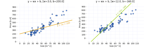
There are two sets of parameters that cause a linear regression model to return different apartment prices for each value of size feature. Because data has a linear pattern, the model could become an accurate approximation of the price after proper calibration of the parameters.
So here’s the question: For which set of parameters does the model return better results?
- Orange:
w = 3,b = 200 - Lime:
w = 12,b = -160
Even though it might be possible to guess the answer just by looking at the graphs, a computer can confirm it numerically. This is where cost function comes into play.
What Is Cost Function?
Cost function measures the performance of a machine learning model for given data. Cost function quantifies the error between predicted and expected values and present that error in the form of a single real number. Depending on the problem, cost function can be formed in many different ways. The purpose of cost function is to be either:
- Minimized: The returned value is usually called cost, error or loss (where loss refers to error for a single data point). The goal is to find the values of model parameters for which cost function return as small a number as possible.
- Maximized: In this case, the value it yields is named a reward. The goal is to find values of model parameters for which the returned number is as large as possible.
For algorithms relying on gradient descent to optimize model parameters, every function has to be differentiable.
How to Tailor a Cost Function
Let’s start with a model using the following formula:
ŷ= predicted value,x= vector of data used for prediction or trainingw= weight.
Notice that we’ve omitted the bias on purpose to simplify the model for visualization. Let’s try to find the value of weight parameter, so for the following data samples:
The outputs of the model are as close as possible to:
Now it’s time to assign a random value to the weight parameter and visualize the model’s results. Let’s pick w = 5.0 for now.
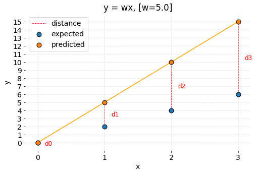
We can observe that the model predictions are different than expected values but how can we express that mathematically? The most straightforward idea is to subtract both values from each other and see if the result of that operation equals zero. Any other result means that the values differ. The size of the received number provides information about how significant the error is. From the geometrical perspective, it’s possible to state that error is the distance between two points in the coordinate system. Let’s define the distance as:
According to the formula, calculate the errors between the predictions and expected values:

As I stated before, cost function is a single number describing model performance. Therefore let’s sum up the errors.

However, now imagine there are a million points instead of four. The accumulated errors will become a bigger number for a model making a prediction on a larger data set than on a smaller data set. Consequently, we can’t compare those models. That’s why we have to scale in some way. The right idea is to divide the accumulated errors by the number of points. Cost stated like that is mean of errors the model made for the given data set.

Unfortunately, the formula isn’t complete. We still have to consider all cases so let’s try picking smaller weights and see if the created cost function works. We’ll set weight to w = 0.5.
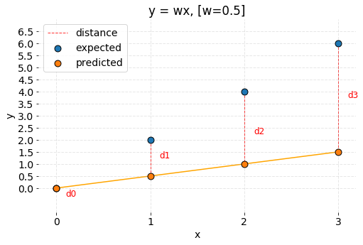
The predictions are off again. However, in comparison to the previous case, that predicted points are below expected points. Numerically, predictions are smaller. The cost formula is going to malfunction because calculated distances have negative values.

The cost value is also negative:
Since distance can’t have a negative value, we can attach a more substantial penalty to the predictions located above or below the expected results (some cost functions do so, e.g. RMSE), but the value shouldn’t be negative because it will cancel out positive errors. It will then become impossible to properly minimize or maximize the cost function. Some cost functions penalize larger errors more heavily, regardless of whether predictions are above or below actual values.
So how about fixing the problem by using the absolute value of the distance? After stating the distance as:
The costs for each value of weights are:

Now we’ve correctly calculated the costs for both weights w = 5.0 and w = 0.5. It is possible to compare the parameters. The model achieves better results for w = 0.5 as the cost value is smaller.
The function we created is mean absolute error.
What Is Mean Absolute Error (MAE)?
Mean absolute error is a regression metric that measures the average magnitude of errors in a group of predictions, without considering their directions. In other words, it’s a mean of absolute differences among predictions and expected results where all individual deviations have even importance.

In this formula:
i= index of sampleŷ= predicted valuey= expected valuem= number of samples in the data set
Sometimes it’s possible to see the form of a formula with swapped predicted and expected values, but it works the same.
Let’s turn math into code:
def mae(predictions, targets):
    # Retrieving number of samples in dataset
    samples_num = len(predictions)

    # Summing absolute differences between predicted and expected values
    accumulated_error = 0.0
    for prediction, target in zip(predictions, targets):
        accumulated_error += np.abs(prediction - target)

    # Calculating mean
    mae_error = (1.0 / samples_num) * accumulated_error

    return mae_error
The function takes as an input two arrays of the same size: predictions and targets. The parameter m of the formula, which is the number of samples, equals the length of sent arrays. Thanks to the fact that arrays have the same length, it’s possible to iterate over both of them at the same time. The absolute value of the difference between each prediction and target is calculated and added to the accumulated_error variable. After gathering errors from all pairs, the accumulated result is averaged by the parameter m that returns MAE error for given data.
What Is Mean Squared Error (MSE)?
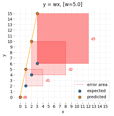
Mean squared error is one of the most commonly used and earliest explained regression metrics. MSE represents the average squared difference between the predictions and expected results. In other words, MSE is an alteration of MAE where, instead of taking the absolute value of differences, we square those differences.
In MAE, the partial error values were equal to the distances between points in the coordinate system. Regarding MSE, each partial error is equivalent to the area of the square created out of the geometrical distance between the measured points. All regional areas are summed up and averaged.
We can write the MSE formula like this:

i= index of sampleŷ= predicted valuey= expected valuem- number of samples in the data set
There are different forms of MSE formula, where there is no division by two in the denominator. Its presence makes MSE derivation calculus cleaner.
Calculating derivatives of equations using absolute value is problematic. MSE uses exponentiation instead and, consequently, has good mathematical properties that make the computation of its derivative easier in comparison to MAE. MSE is more efficient when using a model that relies on the gradient descent algorithm.
We can write MSE in Python as follows:
def mse(predictions, targets):
    # Retrieving number of samples in dataset
    samples_num = len(predictions)

    # Summing square differences between predicted and expected values
    accumulated_error = 0.0
    for prediction, target in zip(predictions, targets):
        accumulated_error += (prediction - target)**2

    # Calculating mean and dividing by 2
    mse_error = (1.0 / (2*samples_num)) * accumulated_error

    return mse_error
The only distinctions from MAE are:
- The difference between prediction and target is squared.
2is in the averaging denominator.
MAE and MSE: Why Do We Use Them So Much?
There are many more regression metrics we can use as cost function for measuring the performance of models that try to solve regression problems (estimating the value). MAE and MSE seem to be relatively simple and very popular.
Why Are There So Many Metrics?
Each metric treats the differences between observations and expected results in a unique way. The distance between ideal result and predictions have a penalty attached by metric, based on the magnitude and direction in the coordinate system. For example, a different metric such as RMSE penalizes all large errors more heavily based on the magnitude, which can make a model prioritize reducing large deviations more aggressively.
So how do MAE and MSE treat the differences between points? To check, let’s calculate the cost for different weight values:

This table presents the errors of many models created with different weight parameters. I calculated the cost of each model with both MAE and MSE metrics.
Here’s how it displays on graphs:
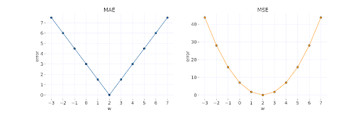
w. Code used to prepare these graphs. | Image: AuthorYou can observe that:
- MAE doesn’t add any additional weight to the distance between points. The error growth is linear.
- MSE errors grow quadratically with distance. It’s a metric that adds a massive penalty to points that are far away and a minimal penalty for points that are close to the expected result. The error curve has a parabolic shape.
Additionally, by checking various weight values, it’s possible to find that the parameter for error is equal to zero. If the w = 2.0 is used to build the model, then the predictions look like this:
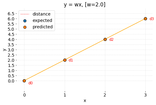
When predictions and expected results overlap, then the value of each reasonable cost function is equal to zero.
Should I Use MSE or MAE?
It’s high time to answer the question about which set of parameters, orange or lime, creates a better approximation for prices of Cracow apartments. Let’s use MSE to calculate the error of both models and see which one is lower.
# Import libraries
import numpy as np
import matplotlib.pyplot as plt
import pandas as pd


# Linear model

def predict(x, parameters):

    return parameters["w"] * x + parameters["b"]

# Load data from .csv
df_data = pd.read_csv("cracow_apartments.csv", sep=",")

# Used features and target value
features = ["size"]
target = ["price"]

# Slice Dataframe to separate feature vectors and target value
X, y = df_data[features].to_numpy(), df_data[target].to_numpy()

# Parameter sets
orange_parameters = {'b': 200, 'w': np.array([3.0])}
lime_parameters = {'b': -160, 'w': np.array([12.0])}

# Make prediction for every data sample
orange_pred = [predict(x, orange_parameters) for x in X]
lime_pred = [predict(x, lime_parameters) for x in X]

# Model error
mse_orange_error = mse(orange_pred, y)
mse_lime_error = mse(lime_pred, y)
Parameters for testing are stored in separate Python dictionaries. Notice that both models use bias this time. We use function predict (x, parameters) for the same data with different parameters. The resulting predictions named orange_pred and lime_pred became an argument for mse (predictions, targets) function, which returned error value for each model separately.
The results are as follows:
- orange: 4909.18
- lime: 10409.77
This means orange parameters create a better model as the cost is smaller.
Frequently Asked Questions
What is a cost function in linear regression?
A cost function in linear regression and machine learning measures the error between a machine learning model’s predicted values and the actual values, helping evaluate and optimize model performance.
What is the difference between MAE and MSE?
MAE (Mean Absolute Error) is a cost function that measures the average absolute difference between predictions and actual results. MSE (Mean Squared Error) is a cost function that squares the differences between predicted and actual values, penalizing larger errors more heavily.


