

Classification is the process of predicting the class of given data points. Classes are sometimes called targets, labels or categories. Classification predictive modeling is the task of approximating a mapping function (f) from input variables (X) to discrete output variables (y.)
What Is Classification in Machine Learning?
For example, spam detection in email service providers can be identified as a classification problem. This is a binary classification since there are only two classes marked as “spam” and “not spam.” A classifier utilizes some training data to understand how given input variables relate to the class. In this case, known spam and non-spam emails have to be used as the training data. When the classifier is trained accurately, it can be used to detect an unknown email.
Classification belongs to the category of supervised learning where the targets are also provided with the input data. Classification can be applied to a wide-variety of tasks, including credit approval, medical diagnosis and target marketing, etc.
Types of Classification in Machine Learning
There are two types of learners in classification — lazy learners and eager learners.
1. Lazy Learners
Lazy learners store the training data and wait until testing data appears. When it does, classification is conducted based on the most related stored training data. Compared to eager learners, lazy learners spend less training time but more time in predicting.
Examples: K-nearest neighbor and case-based reasoning.
2. Eager Learners
Eager learners construct a classification model based on the given training data before receiving data for classification. It must be able to commit to a single hypothesis that covers the entire instance space. Because of this, eager learners take a long time for training and less time for predicting.
Examples: Decision tree, naive Bayes and artificial neural networks.
Classification Algorithms
There are a lot of classification algorithms to choose from. Picking the right one depends on the application and nature of the available data set. For example, if the classes are linearly separable, linear classifiers like logistic regression and Fisher’s linear discriminant can outperform sophisticated models and vice versa.
Important Classification Algorithms to Know
- Decision tree
- Naive Bayes
- Artificial neural network
- K-nearest neighbor (KNN)
Decision Tree
A decision tree builds classification or regression models in the form of a tree structure. It utilizes an “if-then” rule set that is mutually exclusive and exhaustive for classification. The rules are learned sequentially using the training data one at a time. Each time a rule is learned, the tuples covered by the rules are removed. This process continues until it meets a termination condition.
The tree is constructed in a top-down, recursive, divide-and-conquer manner. All attributes should be categorical. Otherwise, they should be discretized in advance. Attributes in the top of the tree have more impact in the classification, and they are identified using the information gain concept.
A decision tree can be easily over-fitted generating too many branches and may reflect anomalies due to noise or outliers. An over-fitted model results in very poor performances on the unseen data, even though it gives off an impressive performance on training data. You can avoid this with pre-pruning, which halts tree construction early, or through post-pruning, which removes branches from the fully grown tree.
Naive Bayes
Naive Bayes is a probabilistic classifier inspired by the Bayes theorem under the assumption that attributes are conditionally independent.
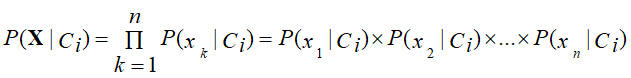
The classification is conducted by deriving the maximum posterior, which is the maximal P(Ci|X), with the above assumption applying to Bayes theorem. This assumption greatly reduces the computational cost by only counting the class distribution. Even though the assumption isn’t valid in most cases since the attributes are dependent, surprisingly, naive Bayes is able to perform impressively.
Naive Bayes is a simple algorithm to implement and can yield good results in most cases. It can be easily scaled to larger data sets since it takes linear time, rather than the expensive iterative approximation that other types of classifiers use.
Naive Bayes can suffer from a problem called the zero probability problem. When the conditional probability is zero for a particular attribute, it fails to give a valid prediction. This needs to be fixed explicitly using a Laplacian estimator.
Artificial Neural Networks
An artificial neural network is a set of connected input/output units, where each connection has a weight associated with it. A team of psychologists and neurobiologists founded it as a way to develop and test computational analogs of neurons. During the learning phase, the network learns by adjusting the weights so as to be able to predict the correct class label of the input tuples.
There are several network architectures available today, including feed-forward, convolutional and recurrent networks. The appropriate architecture depends on the application of the model. For most cases, feed-forward models give reasonably accurate results, but convolutional networks perform better for image processing.
There can be multiple hidden layers in the model depending on the complexity of the function that the model is going to map. These hidden layers will allow you to model complex relationships, such as deep neural networks.
However, when there are many hidden layers, it takes a lot of time to train and adjust the weights. The other disadvantage of this is the poor interpretability of the model compared to others like decision trees. This is due to the unknown symbolic meaning behind the learned weights.
But artificial neural networks have performed impressively in most real world applications. It has a high tolerance for noisy data and is able to classify untrained patterns. Usually, artificial neural networks perform better with continuous-valued inputs and outputs.
All of the above algorithms are eager learners since they train a model in advance to generalize the training data and use it for prediction later.
K-Nearest Neighbor (KNN)
K-Nearest Neighbor is a lazy learning algorithm that stores all instances corresponding to training data points in n-dimensional space. When an unknown discrete data is received, it analyzes the closest k number of instances saved (nearest neighbors) and returns the most common class as the prediction. For real-valued data, it returns the mean of k nearest neighbors.
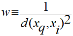
In the distance-weighted nearest neighbor algorithm, it weighs the contribution of each of the k neighbors according to their distance using the following query, giving greater weight to the closest neighbors:
Usually, KNN is robust to noisy data since it is averaging the k-nearest neighbors.
How to Evaluate a Classifier
After training the model, the most important part is to evaluate the classifier to verify its applicability.
Machine Learning Classifier Evaluation Methods
- Holdout method.
- Cross-validation.
- Precision and recall.
- Receiver operating characteristics (ROC) curve.
Holdout Method
There are several methods to evaluate a classifier, but the most common way is the holdout method. In it, the given data set is divided into two partitions, test and train. Twenty percent of the data is used as a test and 80 percent is used to train. The train set will be used to train the model, and the unseen test data will be used to test its predictive power.
Cross-Validation
Overfitting is a common problem in machine learning and it occurs in most models. K-fold cross-validation can be conducted to verify that the model is not overfitted. In this method, the data set is randomly partitioned into k-mutually exclusive subsets, each approximately equal in size. One is kept for testing while others are used for training. This process is iterated throughout the whole k folds.
Precision and Recall
Precision is the fraction of relevant instances among the retrieved instances, while recall is the fraction of relevant instances that have been retrieved over the total amount of relevant instances. Precision and recall are used as a measurement of the relevance.
Receiver Operating Characteristics (ROC) Curve
A ROC curve provides a visual comparison of classification models, showing the trade-off between the true positive rate and the false positive rate.
The area under the ROC curve is a measure of the accuracy of the model. When a model is closer to the diagonal, it is less accurate. A model with perfect accuracy will have an area of 1.0.
Frequently Asked Questions
What are some examples of classification problems?
Examples of classification problems include spam detection, credit approval, medical diagnosis and target marketing.
What are the main types of classification algorithms?
Key algorithms include decision trees, naive Bayes, artificial neural networks and K-nearest neighbor.
What’s the difference between lazy learners and eager learners?
Lazy learners defer model building until prediction time, while eager learners build a model during training.
How do you evaluate a classification model?
Common methods include the holdout method, cross-validation, precision and recall and ROC curves.


