

Regression analysis is a fundamental concept in the field of machine learning. It falls under supervised learning wherein the algorithm is trained with both input features and output labels. It helps in establishing a relationship among the variables by estimating how one variable affects the other.
What Is Regression in Machine Learning?
Imagine you’re car shopping and have decided that gas mileage is a deciding factor in your decision to buy. If you wanted to predict the miles per gallon of some promising rides, how would you do it? Well, since you know the different features of the car (weight, horsepower, displacement, etc.) one possible method is regression. By plotting the average MPG of each car given its features you can then use regression techniques to find the relationship of the MPG and the input features. The regression function here could be represented as $Y = f(X)$, where Y would be the MPG and X would be the input features like the weight, displacement, horsepower, etc. The target function is $f$ and this curve helps us predict whether it’s beneficial to buy or not buy. This mechanism is called regression.
Evaluating a Machine Learning Regression Algorithm
Let’s say you’ve developed an algorithm which predicts next week’s temperature. The temperature to be predicted depends on different properties such as humidity, atmospheric pressure, air temperature and wind speed. But how accurate are your predictions? How good is your algorithm?
To evaluate your predictions, there are two important metrics to be considered: variance and bias.
Variance
Variance is the amount by which the estimate of the target function changes if different training data were used. The target function $f$ establishes the relation between the input (properties) and the output variables (predicted temperature). When a different dataset is used the target function needs to remain stable with little variance because, for any given type of data, the model should be generic. In this case, the predicted temperature changes based on the variations in the training dataset. To avoid false predictions, we need to make sure the variance is low. For that reason, the model should be generalized to accept unseen features of temperature data and produce better predictions.
Bias
Bias is the algorithm’s tendency to consistently learn the wrong thing by not taking into account all the information in the data. For the model to be accurate, bias needs to be low. If there are inconsistencies in the dataset like missing values, less number of data tuples or errors in the input data, the bias will be high and the predicted temperature will be wrong.
The Bias-Variance Trade-off
Accuracy and error are the two other important metrics. The error is the difference between the actual value and the predicted value estimated by the model. Accuracy is the fraction of predictions our model got right.
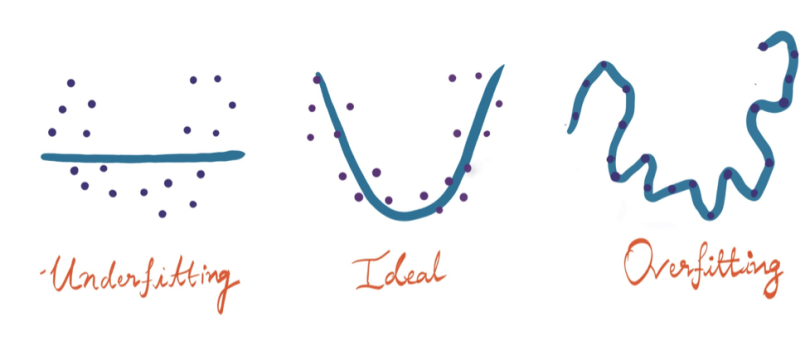
For a model to be ideal, it’s expected to have low variance, low bias and low error. To achieve this, we need to partition the dataset into train and test datasets. The model will then learn patterns from the training dataset and the performance will be evaluated on the test dataset. To reduce the error while the model is learning, we come up with an error function which will be reviewed in the following section. If the model memorizes/mimics the training data fed to it, rather than finding patterns, it will give false predictions on unseen data. The curve derived from the trained model would then pass through all the data points and the accuracy on the test dataset is low. This is called overfitting and is caused by high variance.
On the flip side, if the model performs well on the test data but with low accuracy on the training data, then this leads to underfitting.
There are various algorithms that are used to build a regression model, some work well under certain constraints and some don’t. Before diving into the regression algorithms, let’s see how it works.
Linear Regression in Machine Learning
Linear regression finds the linear relationship between the dependent variable and one or more independent variables using a best-fit straight line. Generally, a linear model makes a prediction by simply computing a weighted sum of the input features, plus a constant called the bias term (also called the intercept term). In this technique, the dependent variable is continuous, the independent variable(s) can be continuous or discrete, and the nature of the regression line is linear. Mathematically, the prediction using linear regression is given as:
$$y = \theta_0 + \theta_1x_1 + \theta_2x_2 + … + \theta_nx_n$$
Here, $y$ is the predicted value,
$n$ is the total number of input features,
$x_i$ is the input feature for $i^{th}$ value,
$\theta_i$ is the model parameter ($\theta_0$ is the bias and the coefficients are $\theta_1, \theta_2, … \theta_n$).
The coefficient is like a volume knob, it varies according to the corresponding input attribute, which brings change in the final value. It signifies the contribution of the input variables in determining the best-fit line.
Bias is a deviation induced to the line equation $y = mx$ for the predictions we make. We need to tune the bias to vary the position of the line that can fit best for the given data.
Drawing the Best-Fit Line
Now, let’s see how linear regression adjusts the line between the data for accurate predictions.
Imagine, you’re given a set of data and your goal is to draw the best-fit line which passes through the data. This is the step-by-step process you proceed with:
- Consider your linear equation to be $y = mx+c$, where y is the dependent data and x is the independent data given in your dataset.
- Adjust the line by varying the values of $m$ and $c$, i.e., the coefficient and the bias.
- Come up with some random values for the coefficient and bias initially and plot the line.
- Since the line won’t fit well, change the values of ‘m’ and ‘c.’ This can be done using the ‘gradient descent algorithm’ or ‘least squares method’.

In accordance with the number of input and output variables, linear regression is divided into three types: simple linear regression, multiple linear regression and multivariate linear regression.
Least Squares Method
First, calculate the error/loss by subtracting the actual value from the predicted one. Since the predicted values can be on either side of the line, we square the difference to make it a positive value. The result is denoted by ‘Q’, which is known as the sum of squared errors.
Mathematically:
$$Q =\sum_{i=1}^{n}(y_{predicted}-y_{original} )^2$$
Our goal is to minimize the error function ‘Q." To get to that, we differentiate Q w.r.t ‘m’ and ‘c’ and equate it to zero. After a few mathematical derivations ‘m’ will be
$$m = \frac{cov(x,y)}{var(x)}$$
And ‘c’ will be,
$$c = y^{-} - bx^{-}$$
By plugging the above values into the linear equation, we get the best-fit line.
Gradient Descent
Gradient descent is an optimization technique used to tune the coefficient and bias of a linear equation.
Imagine you are on the top left of a u-shaped cliff and moving blind-folded towards the bottom center. You take small steps in the direction of the steepest slope. This is what gradient descent does — it is the derivative or the tangential line to a function that attempts to find local minima of a function.
How does gradient descent help in minimizing the cost function?
We take steps down the cost function in the direction of the steepest descent until we reach the minima, which in this case is the downhill. The size of each step is determined by the parameter $\alpha$, called the learning rate. If it’s too big, the model might miss the local minimum of the function, and if it's too small, the model will take a long time to converge. Hence, $\alpha$ provides the basis for finding the local minimum, which helps in finding the minimized cost function.
‘Q’ the cost function is differentiated w.r.t the parameters, $m$ and $c$ to arrive at the updated $m$ and $c$, respectively. The product of the differentiated value and learning rate is subtracted from the actual ones to minimize the parameters affecting the model.
Mathematically, this is how parameters are updated using the gradient descent algorithm:
$$m = m - \alpha\frac{d}{dm}Q$$
$$c = c - \alpha\frac{d}{dc}Q$$
where $Q =\sum_{i=1}^{n}(y_{predicted}-y_{original} )^2$.
This continues until the error is minimized.
Simple Linear Regression in Machine Learning
Simple linear regression is one of the simplest (hence the name) yet powerful regression techniques. It has one input ($x$) and one output variable ($y$) and helps us predict the output from trained samples by fitting a straight line between those variables. For example, we can predict the grade of a student based upon the number of hours they study using simple linear regression.
Mathematically, this is represented by the equation:
$$y = mx +c$$
where $x$ is the independent variable (input),
$y$ is the dependent variable (output),
$m$ is slope,
and $c$ is an intercept.
The above mathematical representation is called a linear equation.
Example: Consider a linear equation with two variables, 3x + 2y = 0.
The values which when substituted make the equation right, are the solutions. For the above equation, (-2, 3) is one solution because when we replace x with -2 and y with +3 the equation holds true and we get 0.
$$3 * -2 + 2 * 3 = 0$$
A linear equation is always a straight line when plotted on a graph.
In simple linear regression, we assume the slope and intercept to be coefficient and bias, respectively. These act as the parameters that influence the position of the line to be plotted between the data.
Imagine you plotted the data points in various colors, below is the image that shows the best-fit line drawn using linear regression.

Multiple Linear Regression in Machine Learning
Multiple linear regression is similar to simple linear regression, but there is more than one independent variable. Every value of the independent variable x is associated with a value of the dependent variable y. As it’s a multi-dimensional representation, the best-fit line is a plane.
Mathematically, it’s expressed by:
$$y = b_0 + b_1x_1 + b_2x_2 + b_3x_3$$
Imagine you need to predict if a student will pass or fail an exam. We’d consider multiple inputs like the number of hours they spent studying, total number of subjects and hours they slept for the previous night. Since we have multiple inputs we would use multiple linear regression.
Multivariate Linear Regression in Machine Learning
As the name implies, multivariate linear regression deals with multiple output variables. For example, if a doctor needs to assess a patient’s health using collected blood samples, the diagnosis includes predicting more than one value, like blood pressure, sugar level and cholesterol level.
Linear Regression in Python Code
# importing boston housing dataset from sklearn
from sklearn.datasets import load_boston
# imports train_test_split to divide the dataset into two parts, one the training set and the other, a test set
from sklearn.model_selection import train_test_split
# importing the LinearRegression model
from sklearn.linear_model import LinearRegression
# matplotlib to visualize the data
import matplotlib.pyplot as plt
data = load_boston()
X_train, X_test, y_train, y_test = train_test_split(data.data, data.target)
clf = LinearRegression()
# training the model using the feature and label
clf.fit(X_train, y_train)
# making predictions on the test data
predicted = clf.predict(X_test)
expected = y_test
# plotting the best-fit line
plt.figure(figsize=(4, 3))
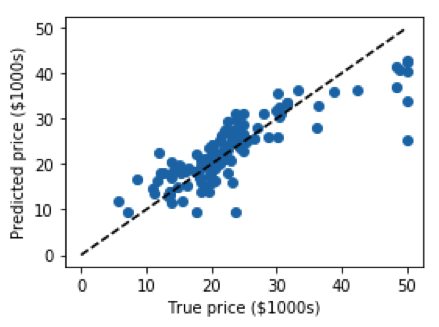
plt.scatter(expected, predicted)
plt.plot([0, 50], [0, 50], '--k')
plt.axis('tight')
plt.xlabel('True price ($1000s)')
plt.ylabel('Predicted price ($1000s)')
plt.tight_layout()Output:
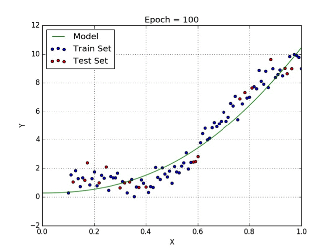
Polynomial Regression in Machine Learning
While the linear regression model is able to understand patterns for a given dataset by fitting in a simple linear equation, it might not might not be accurate when dealing with complex data. In those instances we need to come up with curves which adjust with the data rather than the lines. One approach is to use a polynomial regression model. Here, the degree of the equation we derive from the model is greater than one. Mathematically, a polynomial model is expressed by:
$$Y_{0} = b_{0}+ b_{1}x^{1} + … b_{n}x^{n}$$
where $Y_{0}$ is the predicted value for the polynomial model with regression coefficients $b_{1}$ to $b_{n}$ for each degree and a bias of $b_{0}$.
If n=1, the polynomial equation is said to be a linear equation.
Regularization
Using polynomial regression, we see how the curved lines fit flexibly between the data, but sometimes even these result in false predictions as they fail to interpret the input. For example, if your model is a fifth-degree polynomial equation that’s trying to fit data points derived from a quadratic equation, it will try to update all six coefficients (five coefficients and one bias), which lead to overfitting. Using regularization, we improve the fit so the accuracy is better on the test dataset.
Ridge and Lasso Regression in Machine Learning
To avoid overfitting, we use ridge and lasso regression in the presence of a large number of features. These are the regularization techniques used in the regression field. They work by penalizing the magnitude of coefficients of features along with minimizing the error between the predicted and actual observations. Coefficients evidently increase to fit with a complex model which might lead to overfitting, so when penalized, it puts a check on them to avoid such scenarios.
Ridge regression/L2 regularization adds a penalty term ($\lambda{w_{i}^2}$) to the cost function which avoids overfitting, hence our cost function is now expressed,
$$ J(w) = \frac{1}{n}(\sum_{i=1}^n (\hat{y}(i)-y(i))^2 + \lambda{w_{i}^2})$$
When lambda = 0, we get back to overfitting, and lambda = infinity adds too much weight and leads to underfitting. Therefore, $\lambda$ needs to be chosen carefully to avoid both of these.
In lasso regression/L1 regularization, an absolute value ($\lambda{w_{i}}$) is added rather than a squared coefficient. It stands for least selective shrinkage selective operator.
The cost function would then be:
$$ J(w) = \frac{1}{n}(\sum_{i=1}^n (\hat{y}(i)-y(i))^2 + \lambda{w_{i}})$$
Summary of Machine Learning Regression
- Regression is a supervised machine learning technique which is used to predict continuous values.
- The ultimate goal of the regression algorithm is to plot a best-fit line or a curve between the data.
- The three main metrics that are used for evaluating the trained regression model are variance, bias and error. If the variance is high, it leads to overfitting and when the bias is high, it leads to underfitting.
- Based on the number of input features and output labels, regression is classified as linear (one input and one output), multiple (many inputs and one output) and multivariate (many outputs).
- Linear regression allows us to plot a linear equation, i.e., a straight line. We need to tune the coefficient and bias of the linear equation over the training data for accurate predictions.
- The tuning of coefficient and bias is achieved through gradient descent or a cost function — least squares method.
- Polynomial regression is used when the data is non-linear. In this, the model is more flexible as it plots a curve between the data. The degree of the polynomial needs to vary such that overfitting doesn’t occur.
- Regularization tends to avoid overfitting by adding a penalty term to the cost/loss function.
- Ridge and lasso regression are the techniques which use L2 and L1 regularizations, respectively.
Frequently Asked Questions
What are the three types of regression?
Linear regression, logistic regression and polynomial regression are three common types of regression models used in machine learning. Three main types of regression models used in regression analysis include linear regression, multiple regression and nonlinear regression.
Is regression supervised or unsupervised?
Regression is a supervised machine learning technique that uses an algorithm to analyze the relationship between independent and dependent variables and predict continuous values.
What is the difference between machine learning and regression?
Machine learning is a branch of artificial intelligence (AI) focused on using algorithms to help machines learn without explicit programming. Regression is a statistical method used to measure the relationship between a dependent variable and one or more independent variables.


