Reinforcement Learning With Python: A Guide to Designing and Solving Problems

Reinforcement is a class of machine learning whereby an agent learns how to behave in its environment by performing actions, drawing intuitions and seeing the results. In this article, you’ll learn how to design a reinforcement learning problem and solve it in Python.

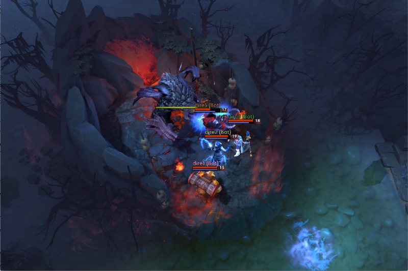
Recently, we’ve been seeing computers playing games against humans, either as bots in multiplayer games or as opponents in one-on-one games like Dota2, PUB-G and Mario. Deepmind made history when its AlphaGo program defeated the South Korean Go world champion in 2016. If you’re an intense gamer, you've probably heard about the Dota 2 OpenAI Five match, where machines played against humans and defeated the world's top Dota2 players in just a few matches. (If you're interested in learning more, here's the complete analysis of the algorithm and the game played by the machine.)

So here’s the central question: Why do we need reinforcement learning? Is it only used for games, or can it be applied to real-world scenarios and problems? The answer: It’s actually one of the most widely used and fastest growing technologies in the field of artificial intelligence.

Here are a few applications that use reinforcement systems:

1. Self driving cars
2. Gaming
3. Robotics
4. Recommendation systems
5. Advertising and marketing

A Brief Review and The Origins of Reinforcement Learning

Where did reinforcement learning come from? Don't we already have plenty of machine learning and deep learning techniques already available?

Reinforcement learning was first proposed by Rich Sutton and Andrew Barto in their Ph.D. thesis (Sutton was the advisor). It took its form in the 1980s but was archaic. Sutton, however, believed its promising nature would lead to eventual recognition.

Reinforcement learning supports automation by learning from the environment it is present in. So too does machine learning and deep learning (different strategies, but both support automation), so why reinforcement learning? Much like the natural learning process, the model receives feedback on whether its performing well or not.

Deep learning and machine learning are learning processes as well, but focus more on finding patterns in the existing data. Reinforcement learning, on the other hand, learns through trial and error, eventually reaching the right actions or the global optimum. A significant additional advantage of reinforcement learning is that only a few chunks of training data are needed, unlike supervised learning, which needs to the whole set.

Understanding Reinforcement Learning

Imagine you're teaching your cat a new trick. Unfortunately, cats don’t understand our language so we can’t tell them what we want them to do. Instead, we emulate a situation and the cat tries to respond in different ways. If the cat’s response is the desired one, we reward them with milk, and guess what? The next time the cat is exposed to the same situation, it executes a similar action with even more enthusiasm in expectation of more food. So this is learning from positive responses.

Similarly, this is how reinforcement learning works — we give the machines a few inputs and actions and then reward them based on the output. Reward maximization will be our end goal. Now let’s see how we interpret the same problem above as a reinforcement learning problem.

• The cat will be the “agent” that is exposed to the “environment.”
• The environment is a house/play-area depending on what you're teaching.
• The situation encountered is called the “state,” which is analogous for example, to your cat crawling under the bed or running. These can be interpreted as states.
• The agents react by performing actions to change from one “state” to another.
• After the change in states, we give the agent either a “reward” or a “penalty” depending on the action that is performed.
• The “policy” is the strategy of choosing an action for finding better outcomes.

Now that we understand the basics of reinforcement learning, let’s deep dive into the origins and evolution of reinforcement learning and deep reinforcement learning and how they can solve problems that supervised or unsupervised learning can’t. (Fun fact: Google's search engine is optimized using reinforcement algorithms.)

Getting familiar with Reinforcement Learning Terminology

Agent and the environment play the essential role in the reinforcement learning algorithm. The environment is the world that agent survives in. The agent also perceives a reward signal from the environment, a number that tells it how good or bad the current world state is. The goal of the agent is to maximize its cumulative reward, called return. Before we write our first reinforcement learning algorithms, we need to understand the following terminology:

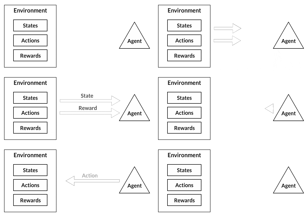
1. States: The state is a complete description of the world. No piece of information present in the world is hidden. It can be a position, a constant or a dynamic. We mostly record these states in arrays, matrices or higher order tensors.
2. Action: Action is usually based on the environment, different environments lead to different actions based on the agent. Set of valid actions for an agent are recorded in a space called an action space. These are usually finite in number.
3. Environment: This is the place where the agent lives and interacts. For different types of environments, we use different rewards, policies, etc.
4. Reward and return: The reward function R is the one which must be tracked all the time in reinforcement learning. It plays a vital role in tuning, optimizing the algorithm and stop training the algorithm. It depends on the current state of the world, the action just taken, and the next state of the world.
5. Policies: Policy is a rule used by an agent for choosing the next action. These are also called the agent's brains.

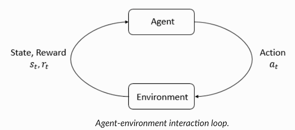
Before solving a problem using reinforcement algorithms, we must understand how to design an issue and assign the reinforcement learning terminology we just learned.

Solving the Taxi Problem

Imagine we're teaching a taxi how to transport people in a parking lot to four different locations (R,G,Y,B) . The first step is to set up a Python environment (if you're new to Python, I recommend this article).

You can setup up the taxi-problem environment using OpenAi’s Gym, which is one of the most used libraries for solving reinforcement problems. To install the library, use the Python package installer (pip):

pip install gym

Now let’s see how our environment is going to render. All the models and interface for this problem are already configured in Gym and named under Taxi-V2. Use the code snippet below to render this environment:

“There are 4 locations (labelled by different letters), and our job is to pick up the passenger at one location and drop him off at another. We receive +20 points for a successful drop-off and lose 1 point for every time-step it takes. There is also a 10 point penalty for illegal pick-up and drop-off actions.” (Source: https://gym.openai.com/envs/Taxi-v2/ )

This will be the rendered output on your console:

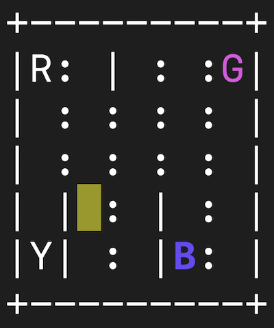
Perfect. Env is the core of OpenAi Gym, which is the unified environment interface. The following are the env methods that will be quite helpful to us:

env.reset: Resets the environment and returns a random initial state.
env.step(action): Step the environment by one timestep.
env.step(action): Returns the following variables:

• observation: Observations of the environment.
• reward: If your action was beneficial or not.
• done: Indicates if we have successfully picked up and dropped off a passenger, also called one episode.
• info: Additional info such as performance and latency for debugging purposes.
• env.render: Renders one frame of the environment (helpful in visualizing the environment).

Now that we have seen the environment, let’s dive deeper in breaking down the problem. The taxi is the only car in this parking lot. We can break the parking lot into a 5x5 grid, which gives us 25 possible taxi locations. These 25 locations are one part of our state space. Notice the current location state of our taxi is coordinate (3, 1).

In the environment, there are four possible locations where you can drop off the passengers: R, G, Y, B or [(0,0), (0,4), (4,0), (4,3)]in (row, col) coordinates if you can interpret the above-rendered environment as a coordinate axis.

When we also account for one (1) additional passenger state of being inside the taxi, we can take all combinations of passenger locations and destination locations to come to a total number of states for our taxi environment — there are four (4) destinations and five (4 + 1) passenger locations. So, our taxi environment has 5×5×5×4=500 total possible states. The agent encounters one of the 500 states, and it takes action. The action in our case can be to move in a direction or decide to pick up/drop off a passenger.

In other words, we have six possible actions: pickup, drop, north, east,south, west(These four directions are the moves by which the taxi is moved.)

This is the action space: the set of all the actions that our agent can take in a given state.

You’ll notice in the illustration above, that the taxi cannot perform certain actions in certain states due to walls. In the environment’s code, we will simply provide a -1 penalty for every wall hit and the taxi won’t move anywhere. This will just rack up penalties causing the taxi to consider going around the wall.

Reward Table: When the taxi environment is created, there is an initial reward table that’s also created, called P. We can think of it like a matrix that has the number of states as rows and number of actions as columns, i.e. states × actions matrix.

Since every state is in this matrix, we can see the default reward values assigned to our illustration’s state:

>>> import gym
>>> env = gym.make("Taxi-v2").env
>>> env.P[328]
{0: [(1.0, 433, -1, False)], 
 1: [(1.0, 233, -1, False)],
 2: [(1.0, 353, -1, False)],
 3: [(1.0, 333, -1, False)],
 4: [(1.0, 333, -10, False)],
 5: [(1.0, 333, -10, False)]
}

This dictionary has a structure {action: [(probability, nextstate, reward, done)]}.

• The 0–5 corresponds to the actions (south, north, east, west, pickup, drop off) the taxi can perform at our current state in the illustration.
• done is used to tell us when we have successfully dropped off a passenger in the right location.

To solve the problem without any reinforcement learning, we can set the goal state, choose some sample spaces and then if it reaches the goal state with a number of iterations we assume it’s the maximum reward, else the reward is increased if it’s near to goal state and penalty is raised if reward for the step is -10 which is minimum.

Now let’s code this problem without reinforcement learning.

Since we have our P table for default rewards in each state, we can try to have our taxi navigate just using that.

We’ll create an infinite loop which runs until one passenger reaches one destination (one episode), or in other words, when the received reward is 20. The env.action_space.sample()method automatically selects one random action from set of all possible actions.

Let’s see what happens:

taxi-nrl.py on GitHub

import gym
from time import sleep

# Creating thr env
env = gym.make("Taxi-v2").env

env.s = 328


# Setting the number of iterations, penalties and reward to zero,
epochs = 0
penalties, reward = 0, 0

frames = []

done = False

while not done:
    action = env.action_space.sample()
    state, reward, done, info = env.step(action)

    if reward == -10:
        penalties += 1

    # Put each rendered frame into the dictionary for animation
    frames.append({
        'frame': env.render(mode='ansi'),
        'state': state,
        'action': action,
        'reward': reward
    }
    )

    epochs += 1

print("Timesteps taken: {}".format(epochs))
print("Penalties incurred: {}".format(penalties))

# Printing all the possible actions, states, rewards.
def frames(frames):
    for i, frame in enumerate(frames):
        clear_output(wait=True)
        print(frame['frame'].getvalue())
        print(f"Timestep: {i + 1}")
        print(f"State: {frame['state']}")
        print(f"Action: {frame['action']}")
        print(f"Reward: {frame['reward']}")
        sleep(.1)
        
frames(frames)

Output:

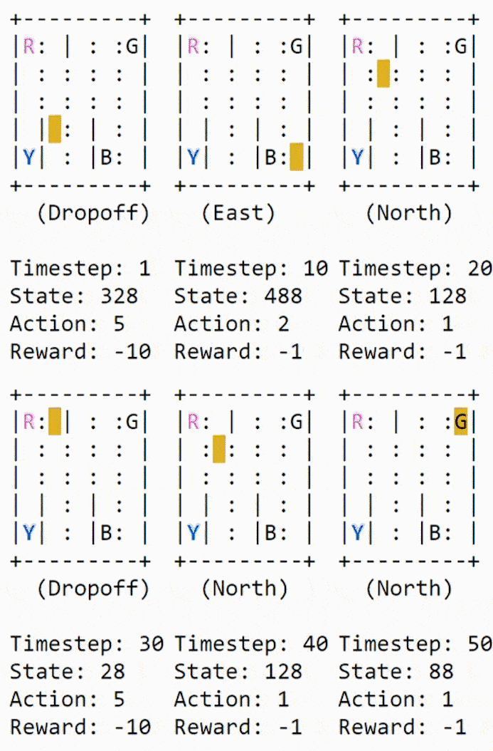
Our problem is solved, but isn’t optimized because this algorithm doesn’t work all the time. We need a proper interacting agent so the number of iterations that the machine/algorithm takes is much less. Luckily, we can use the Q-learning algorithm.

Introduction to Q-Learning

The Q-learning algorithm is most used as a basic reinforcement algorithm. It  uses the environment rewards to learn over time the best action to take in a given state. In the above implementation, we have our reward table “P” from where the agent will learn. Using the reward table it chooses the next action if it’s beneficial or not and then updates a new value called the Q-value. The newly created table is called the Q-table and maps to a combination called (state, action) combination. If the Q-values are better, we have more optimized rewards.

For example, if the taxi is faced with a state that includes a passenger at its current location, it is highly likely that the Q-value for pickup is higher when compared to other actions, like drop off or north.

Q-values are initialized to an arbitrary value, and as the agent exposes itself to the environment and receives different rewards by executing different actions, the Q-values are updated using the equation:

How do we initialize the Q-values and calculate them? For that, we initialize the Q-values with arbitrary constants. As the agent is exposed to the environment, it receives various rewards by executing different actions. Once the actions are executed, the Q-values are executed by the equation.

Here alpha and gamma are the parameters for the Q-learning algorithm. Alpha is known as the learning rate and gamma as the discount factor. Both values range between 0 and 1 and sometimes equal to one. Gamma can be zero while alpha cannot, as the loss should be updated with some learning rate. Here alpha here represents the same which is used in supervised learning. Gamma determines how much importance we want to give to future rewards.

Below is the algorithm in brief:

• Step 1: Initialize the Q-table with all zeros and Q-values to arbitrary constants.
• Step 2: Let the agent react to the environment and explore the actions. For each change in state, select any one among all possible actions for the current state (S).
• Step 3: Travel to the next state (S’) as a result of that action (a).
• Step 4: For all possible actions from the state (S’) select the one with the highest Q-value.
• Step 5: Update Q-table values using the equation.
• State 6: Change the next state as the current state.
• Step 7: If goal state is reached, then end and repeat the process.

Q-Learning in Python

q-learning.py on GitHub

import gym
import numpy as np
import random
from IPython.display import clear_output

# Init Taxi-V2 Env
env = gym.make("Taxi-v2").env

# Init arbitary values
q_table = np.zeros([env.observation_space.n, env.action_space.n])

# Hyperparameters
alpha = 0.1
gamma = 0.6
epsilon = 0.1


all_epochs = []
all_penalties = []

for i in range(1, 100001):
    state = env.reset()

    # Init Vars
    epochs, penalties, reward, = 0, 0, 0
    done = False

    while not done:
        if random.uniform(0, 1) < epsilon:
            # Check the action space
            action = env.action_space.sample()
        else:
            # Check the learned values
            action = np.argmax(q_table[state])

        next_state, reward, done, info = env.step(action)

        old_value = q_table[state, action]
        next_max = np.max(q_table[next_state])

        # Update the new value
        new_value = (1 - alpha) * old_value + alpha * \
            (reward + gamma * next_max)
        q_table[state, action] = new_value

        if reward == -10:
            penalties += 1

        state = next_state
        epochs += 1

    if i % 100 == 0:
        clear_output(wait=True)
        print("Episode: {i}")

print("Training finished.")

That's it. Your model is trained and the environment can now drop the passengers more accurately.

More Reinforcement Techniques

• MDPs and Bellman Equations
• Dynamic Programming: Model-Based RL, Policy Iteration and Value Iteration
• Deep Q Learning
• Policy Gradient Methods
• SARSA

Code for this article can be found on GitHub.

_{^{References: OpenAI, Playing Atari with Deep Reinforcement Learning, SkyMind, LearnDataSci.}}

RelatedRead More About Data Science