Unsupervised learning is a class of machine learning (ML) techniques used to find patterns in data. The data given to unsupervised algorithms is not labelled, which means only the input variables (x) are given with no corresponding output variables. In unsupervised learning, the algorithms are left to discover interesting structures in the data on their own.
Yan Lecun, VP and chief AI scientist at Facebook, has said unsupervised learning — teaching machines to learn for themselves without the need to be explicitly told if everything they do is right or wrong — is the key to “true AI.”
Unsupervised Learning
Supervised vs. Unsupervised Learning
In supervised learning, the system tries to learn from the previous examples given. In unsupervised learning, the system attempts to find the patterns directly from the example given. So, if the dataset is labeled it is a supervised problem, and if the dataset is unlabelled then it is an unsupervised problem.
Below is a simple pictorial representation of how supervised and unsupervised learning can be viewed.
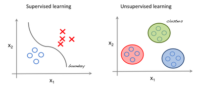
The left image an example of supervised learning (we use regression techniques to find the best fit line between the features). In unsupervised learning the inputs are segregated based on features and the prediction is based on which cluster it belonged to.
Important Terminology
-
Feature: An input variable used in making predictions.
-
Predictions: A model’s output when provided with an input example.
-
Example: One row of a dataset. An example contains one or more features and possibly a label.
- Label: Result of the feature.
Preparing Data for Unsupervised Learning
For our example, we'll use the Iris dataset to make predictions. The dataset contains a set of 150 records under four attributes — petal length, petal width, sepal length, sepal width, and three iris classes: setosa, virginica and versicolor. We'll feed the four features of our flower to the unsupervised algorithm and it will predict which class the iris belongs to.
We use the scikit-learn library in Python to load the Iris dataset and matplotlib for data visualization. Below is the code snippet for exploring the dataset.
On GitHub: iris_dataset.py
# Importing Modules
from sklearn import datasets
import matplotlib.pyplot as plt

# Loading dataset
iris_df = datasets.load_iris()

# Available methods on dataset
print(dir(iris_df))

# Features
print(iris_df.feature_names)

# Targets
print(iris_df.target)

# Target Names
print(iris_df.target_names)
label = {0: 'red', 1: 'blue', 2: 'green'}

# Dataset Slicing
x_axis = iris_df.data[:, 0]  # Sepal Length
y_axis = iris_df.data[:, 2]  # Sepal Width

# Plotting
plt.scatter(x_axis, y_axis, c=iris_df.target)
plt.show()
['DESCR', 'data', 'feature_names', 'target', 'target_names']
['sepal length (cm)', 'sepal width (cm)', 'petal length (cm)', 'petal width (cm)']
[0 0 0 0 0 0 0 0 0 0 0 0 0 0 0 0 0 0 0 0 0 0 0 0 0 0 0 0 0 0 0 0 0 0 0 0 0 0 0 0 0 0 0 0 0 0 0 0 0 0 1 1 1 1 1 1 1 1 1 1 1 1 1 1 1 1 1 1 1 1 1 1 1 1 1 1 1 1 1 1 1 1 1 1 1 1 1 1 1 1 1 1 1 1 1 1 1 1 1 1 2 2 2 2 2 2 2 2 2 2 2 2 2 2 2 2 2 2 2 2 2 2 2 2 2 2 2 2 2 2 2 2 2 2 2 2 2 2 2 2 2 2 2 2 2 2 2 2 2 2]
['setosa' 'versicolor' 'virginica']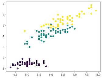
Clustering
In clustering, the data is divided into several groups with similar traits.

In the image above, the left is raw data without classification, while the right is clustered based on its features. When an input is given which is to be predicted then it checks in the cluster it belongs to based on its features, and the prediction is made.
K-Means Clustering in Python
K-means clustering is an iterative unsupervised clustering algorithm that aims to find local maxima in each iteration. Initially, desired number of clusters are chosen. In our example, we know there are three classes involved, so we program the algorithm to group the data into three classes by passing the parameter “n_clusters” into our k-means model. Randomly, three points (inputs) are assigned into three clusters. Based on the centroid distance between each point, the next given inputs are segregated into respected clusters and the centroids are re-computed for all the clusters.
Each centroid of a cluster is a collection of feature values which define the resulting groups. Examining the centroid feature weights can be used to qualitatively interpret what kind of group each cluster represent.
We import the k-means model from scikit-learn library, fit out features and predict.
K-means implementation in Python on GitHub: clustering_iris.py
# Importing Modules
from sklearn import datasets
from sklearn.cluster import KMeans

# Loading dataset
iris_df = datasets.load_iris()

# Declaring Model
model = KMeans(n_clusters=3)

# Fitting Model
model.fit(iris_df.data)

# Predicitng a single input
predicted_label = model.predict([[7.2, 3.5, 0.8, 1.6]])

# Prediction on the entire data
all_predictions = model.predict(iris_df.data)

# Printing Predictions
print(predicted_label)
print(all_predictions)
[0]
[0 0 0 0 0 0 0 0 0 0 0 0 0 0 0 0 0 0 0 0 0 0 0 0 0 0 0 0 0 0 0 0 0 0 0 0 0 0 0 0 0 0 0 0 0 0 0 0 0 0 2 2 1 2 2 2 2 2 2 2 2 2 2 2 2 2 2 2 2 2 2 2 2 2 2 2 2 1 2 2 2 2 2 2 2 2 2 2 2 2 2 2 2 2 2 2 2 2 2 2 1 2 1 1 1 1 2 1 1 1 1 1 1 2 2 1 1 1 1 2 1 2 1 2 1 1 2 2 1 1 1 1 1 2 1 1 1 1 2 1 1 1 2 1 1 1 2 1 1 2]Hierarchical Clustering
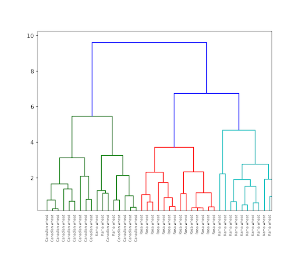
As its name implies, hierarchical clustering is an algorithm that builds a hierarchy of clusters. This algorithm begins with all the data assigned to a cluster, then the two closest clusters are joined into the same cluster. The algorithm ends when only a single cluster is left.
The completion of hierarchical clustering can be shown using dendrogram. Now let’s look at an example of hierarchical clustering using grain data. The dataset can be found here.
Hierarchical clustering implementation in Python on GitHub: hierchical-clustering.py
# Importing Modules
from scipy.cluster.hierarchy import linkage, dendrogram
import matplotlib.pyplot as plt
import pandas as pd

# Reading the DataFrame
seeds_df = pd.read_csv(
    "https://raw.githubusercontent.com/vihar/unsupervised-learning-with-python/master/seeds-less-rows.csv")

# Remove the grain species from the DataFrame, save for later
varieties = list(seeds_df.pop('grain_variety'))

# Extract the measurements as a NumPy array
samples = seeds_df.values

"""
Perform hierarchical clustering on samples using the
linkage() function with the method='complete' keyword argument.
Assign the result to mergings.
"""
mergings = linkage(samples, method='complete')

"""
Plot a dendrogram using the dendrogram() function on mergings,
specifying the keyword arguments labels=varieties, leaf_rotation=90,
and leaf_font_size=6.
"""
dendrogram(mergings,
           labels=varieties,
           leaf_rotation=90,
           leaf_font_size=6,
           )

plt.show()
Difference between K-Means and Hierarchical clustering
- Hierarchical clustering can’t handle big data very well but k-means clustering can. This is because the time complexity of k-means is linear i.e. O(n) while that of hierarchical clustering is quadratic i.e. O(n2).
- K-means clustering starts with an arbitrary choice of clusters, and the results generated by running the algorithm multiple times might differ. Results are reproducible in hierarchical clustering.
- K-means is found to work well when the shape of the clusters is hyperspherical (like a circle in 2D or a sphere in 3D).
- K-means doesn't allow noisy data, while hierarchical clustering can directly use the noisy dataset for clustering.
t-SNE Clustering
One of the unsupervised learning methods for visualization is t-distributed stochastic neighbor embedding, or t-SNE. It maps high-dimensional space into a two or three-dimensional space which can then be visualized. Specifically, it models each high-dimensional object by a two- or three-dimensional point in such a way that similar objects are modeled by nearby points and dissimilar objects are modeled by distant points with high probability.
T-SNE Implementation in Python on Iris dataset: t_sne_clustering.py
# Importing Modules
from sklearn import datasets
from sklearn.manifold import TSNE
import matplotlib.pyplot as plt

# Loading dataset
iris_df = datasets.load_iris()

# Defining Model
model = TSNE(learning_rate=100)

# Fitting Model
transformed = model.fit_transform(iris_df.data)

# Plotting 2d t-Sne
x_axis = transformed[:, 0]
y_axis = transformed[:, 1]

plt.scatter(x_axis, y_axis, c=iris_df.target)
plt.show()
Here, the Iris dataset has four features (4d) and is transformed and represented in the two-dimensional figure. Similarly, t-SNE model can be applied to a dataset which has n-features.
DBSCAN Clustering
Density-based spatial clustering of applications with noise, or DBSCAN, is a popular clustering algorithm used as a replacement for k-means in predictive analytics. To run it doesn’t require an input for the number of clusters but it does need to tune two other parameters.
The scikit-learn implementation provides a default for the eps and min_samples parameters, but you’re generally expected to tune those. The eps parameter is the maximum distance between two data points to be considered in the same neighborhood. The min_samples parameter is the minimum amount of data points in a neighborhood to be considered a cluster.
DBSCAN clustering in Python on GitHub: dbscan.py
# Importing Modules
from sklearn.datasets import load_iris
import matplotlib.pyplot as plt
from sklearn.cluster import DBSCAN
from sklearn.decomposition import PCA

# Load Dataset
iris = load_iris()

# Declaring Model
dbscan = DBSCAN()

# Fitting
dbscan.fit(iris.data)

# Transoring Using PCA
pca = PCA(n_components=2).fit(iris.data)
pca_2d = pca.transform(iris.data)

# Plot based on Class
for i in range(0, pca_2d.shape[0]):
    if dbscan.labels_[i] == 0:
        c1 = plt.scatter(pca_2d[i, 0], pca_2d[i, 1], c='r', marker='+')
    elif dbscan.labels_[i] == 1:
        c2 = plt.scatter(pca_2d[i, 0], pca_2d[i, 1], c='g', marker='o')
    elif dbscan.labels_[i] == -1:
        c3 = plt.scatter(pca_2d[i, 0], pca_2d[i, 1], c='b', marker='*')

plt.legend([c1, c2, c3], ['Cluster 1', 'Cluster 2', 'Noise'])
plt.title('DBSCAN finds 2 clusters and Noise')
plt.show()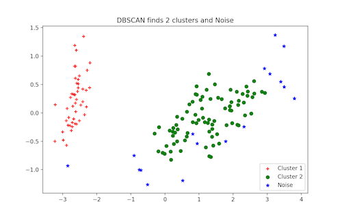
Related Unsupervised Learning Video
More Unsupervised Learning Techniques
- Principal component analysis (PCA)
- Autoencoders
- Deep belief nets
- Hebbian learning
- Generative adversarial networks (GANs)
- Self-organizing maps