Have you ever wondered how Google can translate entire paragraphs from one language into another in a matter of milliseconds; how Netflix and YouTube can provide good recommendations; how self-driving cars are even possible?
All of these innovations are the product of deep learning and artificial neural networks.
What Is Deep Learning?
Deep learning is just a type of machine learning, inspired by the structure of the human brain. Deep learning algorithms attempt to draw similar conclusions as humans would by continually analyzing data with a given logical structure. To achieve this, deep learning uses multi-layered structures of algorithms called neural networks.
What Is Deep Learning?
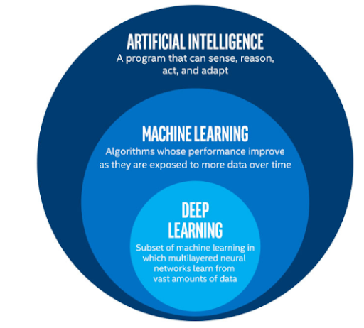
Deep learning is a subset of machine learning, which is a subset of artificial intelligence. Artificial intelligence is a general term that refers to techniques that enable computers to mimic human behavior. Machine learning represents a set of algorithms trained on data that make all of this possible. Deep learning is just a type of machine learning, inspired by the structure of the human brain.
How Does Deep Learning Work?
Deep learning algorithms attempt to draw similar conclusions as humans would by constantly analyzing data with a given logical structure. To achieve this, deep learning uses a multi-layered structure of algorithms called neural networks.
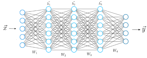
The design of the neural network is based on the structure of the human brain. Just as we use our brains to identify patterns and classify different types of information, we can teach neural networks to perform the same tasks on data.
The individual layers of neural networks can also be thought of as a sort of filter that works from gross to subtle, which increases the likelihood of detecting and outputting a correct result. The human brain works similarly. Whenever we receive new information, the brain tries to compare it with known objects. The same concept is also used by deep neural networks.
Neural networks enable us to perform many tasks, such as clustering, classification or regression.
With neural networks, we can group or sort unlabeled data according to similarities among samples in the data. Or, in the case of classification, we can train the network on a labeled data set in order to classify the samples in the data set into different categories.
In general, neural networks can perform the same tasks as classical machine learning algorithms (but classical algorithms cannot perform the same tasks as neural networks). In other words, artificial neural networks have unique capabilities that enable deep learning models to solve tasks that machine learning models can never solve.
All recent advances in artificial intelligence in recent years are due to deep learning. Without deep learning, we would not have self-driving cars, chatbots or personal assistants like Alexa and Siri. Google Translate would continue to be as primitive as it was before Google switched to neural networks and Netflix would have no idea which movies to suggest. Neural networks are behind all of these deep learning applications and technologies.
A new industrial revolution is taking place, driven by artificial neural networks and deep learning. At the end of the day, deep learning is the best and most obvious approach to real machine intelligence we’ve ever had.
Why Is Deep Learning Popular?
Deep learning models are more powerful than machine learning models but why?
No Feature Extraction
The first advantage of deep learning over machine learning is the redundancy of the so-called feature extraction.
Long before we began using deep learning, we relied on traditional machine learning methods including decision trees, SVM, naïve Bayes classifier and logistic regression. These algorithms are also called flat algorithms. “Flat” here refers to the fact these algorithms cannot normally be applied directly to the raw data (such as .csv, images, text, etc.). We need a preprocessing step called feature extraction.
The result of feature extraction is a representation of the given raw data that these classic machine learning algorithms can use to perform a task. For example, we can now classify the data into several categories or classes. Feature extraction is usually quite complex and requires detailed knowledge of the problem domain. This preprocessing layer must be adapted, tested and refined over several iterations for optimal results.
Deep learning’s artificial neural networks don’t need the feature extraction step. The layers are able to learn an implicit representation of the raw data directly and on their own.
Here’s how it works: A more and more abstract and compressed representation of the raw data is produced over several layers of an artificial neural net. We then use this compressed representation of the input data to produce the result. The result can be, for example, the classification of the input data into different classes.
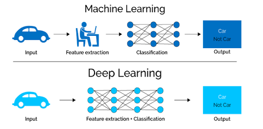
In other words, we can say that the feature extraction step is already part of the process that takes place in an artificial neural network.
During the training process, this neural network optimizes this step to obtain the best possible abstract representation of the input data. This means that deep learning models require little to no manual effort to perform and optimize the feature extraction process.
Let’s look at a concrete example. If you want to use a machine learning model to determine if a particular image is showing a car or not, we humans first need to identify the unique features of a car (shape, size, windows, wheels, etc.), then extract the feature and give it to the algorithm as input data. In this way, the algorithm would perform a classification of the images. That is, in machine learning, a programmer must intervene directly in the action for the model to come to a conclusion.
In the case of a deep learning model, the feature extraction step is completely unnecessary. The model would recognize these unique characteristics of a car and make correct predictions without human intervention.
In fact, refraining from extracting the characteristics of data applies to every other task you’ll ever do with neural networks. Simply give the raw data to the neural network and the model will do the rest.
Deep Learning Accuracy Can Increase By Using Big Data
The second huge advantage of deep learning, and a key part of understanding why it’s becoming so popular, is that it’s powered by massive amounts of data. The era of big data will provide huge opportunities for new innovations in deep learning. But don’t take my word for it Andrew Ng, the chief scientist of China’s major search engine Baidu, co-founder of Coursera and one of the leaders of the Google Brain Project, puts it this way:
I think AI is akin to building a rocket ship. You need a huge engine and a lot of fuel. If you have a large engine and a tiny amount of fuel, you won’t make it to orbit. If you have a tiny engine and a ton of fuel, you can’t even lift off. To build a rocket you need a huge engine and a lot of fuel.
The analogy to deep learning is that the rocket engine is the deep learning models and the fuel is the huge amounts of data we can feed to these algorithms.
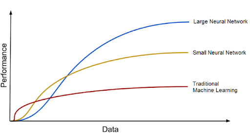
Deep learning models tend to increase their accuracy with the increasing amount of training data, whereas traditional machine learning models such as SVM and naive Bayes classifier stop improving after a saturation point.
How Do Deep Learning Neural Networks Work?
Biological Neural Networks
Artificial neural networks are inspired by the biological neurons found in our brains. In fact, the artificial neural networks simulate some basic functionalities of biological neural network, but in a very simplified way. Let’s first look at the biological neural networks to derive parallels to artificial neural networks.
In short, a biological neural network consists of numerous neurons.
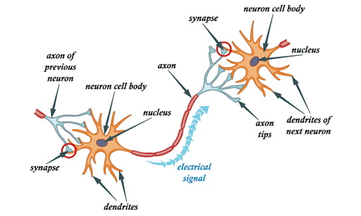
A typical neuron consists of a cell body, dendrites and an axon. Dendrites are thin structures that emerge from the cell body. An axon is a cellular extension that emerges from this cell body. Most neurons receive signals through the dendrites and send out signals along the axon.
At the majority of synapses, signals cross from the axon of one neuron to the dendrite of another. All neurons are electrically excitable due to the maintenance of voltage gradients in their membranes. If the voltage changes by a large enough amount over a short interval, the neuron generates an electrochemical pulse called an action potential. This potential travels rapidly along the axon and activates synaptic connections.
Artificial Neural Networks
Now that we have a basic understanding of how biological neural networks are functioning, let’s take a look at the architecture of the artificial neural network.
A neural network generally consists of a collection of connected units or nodes. We call these nodes neurons. These artificial neurons loosely model the biological neurons of our brain.
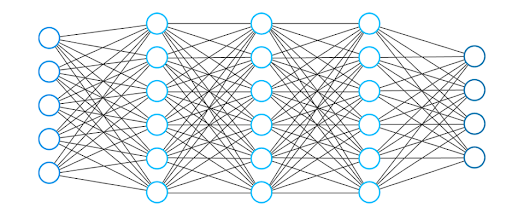
A neuron is simply a graphical representation of a numeric value (e.g. 1.2, 5.0, 42.0, 0.25, etc.). Any connection between two artificial neurons can be considered an axon in a biological brain. The connections between the neurons are realized by so-called weights, which are also nothing more than numerical values.
When an artificial neural network learns, the weights between neurons change, as does the strength of the connection. Well what does that mean? Given training data and a particular task such as classification of numbers, we are looking for certain set weights that allow the neural network to perform the classification.
The set of weights is different for every task and every data set. We cannot predict the values of these weights in advance, but the neural network has to learn them. The process of learning is what we call training.
Deep Learning Neural Network Architecture
The typical neural network architecture consists of several layers; we call the first one the input layer.
The input layer receives input x, (i.e. data from which the neural network learns). In our previous example of classifying handwritten numbers, these inputs x would represent the images of these numbers (x is basically an entire vector where each entry is a pixel).
The input layer has the same number of neurons as there are entries in the vector x. In other words, each input neuron represents one element in the vector.
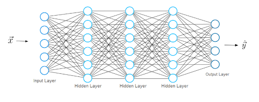
The last layer is called the output layer, which outputs a vector y representing the neural network’s result. The entries in this vector represent the values of the neurons in the output layer. In our classification, each neuron in the last layer represents a different class.
In this case, the value of an output neuron gives the probability that the handwritten digit given by the features x belongs to one of the possible classes (one of the digits 0-9). As you can imagine the number of output neurons must be the same number as there are classes.
In order to obtain a prediction vector y, the network must perform certain mathematical operations, which it performs in the layers between the input and output layers. We call these the hidden layers. Now let's discuss what the connections between the layers look like.
Layer Connections in a Deep Learning Neural Network
Please consider a smaller neural network that consists of only two layers. The input layer has two input neurons, while the output layer consists of three neurons.
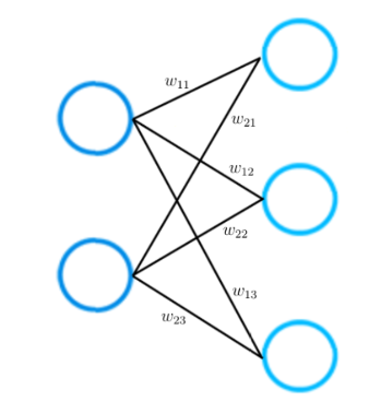
As mentioned earlier, each connection between two neurons is represented by a numerical value, which we call weight.
As you can see in the picture, each connection between two neurons is represented by a different weight w. Each of these weight w has indices. The first value of the indices stands for the number of neurons in the layer from which the connection originates, the second value for the number of the neurons in the layer to which the connection leads.
All weights between two neural network layers can be represented by a matrix called the weight matrix.
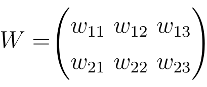
A weight matrix has the same number of entries as there are connections between neurons. The dimensions of a weight matrix result from the sizes of the two layers that are connected by this weight matrix.
The number of rows corresponds to the number of neurons in the layer from which the connections originate and the number of columns corresponds to the number of neurons in the layer to which the connections lead.
In this particular example, the number of rows of the weight matrix corresponds to the size of the input layer, which is two, and the number of columns to the size of the output layer, which is three.
Learning a Deep Learning Neural Network’s Process
Now that we understand the neural network architecture better, we can better study the learning process. Let’s do it step-by-step. You already know step one. For a given input feature vector x, the neural network calculates a prediction vector, which we call h.
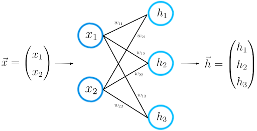
We also call this step forward propagation. With the input vector x and the weight matrix W connecting the two neuron layers, we compute the dot product between the vector x and the matrix W.
The result of this dot product is another vector, which we call z.
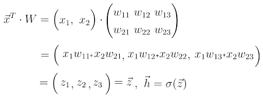
We obtain the final prediction vector h by applying a so-called activation function to the vector z. In this case, the activation function is represented by the letter sigma.
An activation function is only a nonlinear function that performs a nonlinear mapping from z to h.
There are three activation functions we use in deep learning: tanh, sigmoid and ReLu.
At this point, you may recognize the meaning behind neurons in a neural network: simply a representation of a numeric value. Let’s take a closer look at vector z for a moment.
As you can see, each element of z consists of the input vector x. At this point, the role of the weights unfold beautifully. A value of a neuron in a layer consists of a linear combination of neuron values of the previous layer weighted by some numeric values.
These numerical values are the weights that tell us how strongly these neurons are connected with each other.
During training, these weights adjust; some neurons become more connected while some neurons become less connected. As in a biological neural network, learning means weight alteration. Accordingly, the values of z, h and the final output vector y are changing with the weights. Some weights make the predictions of a neural network closer to the actual ground truth vector y_hat; other weights increase the distance to the ground truth vector.
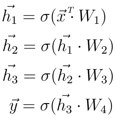
Now that we know what the mathematical calculations between two neural network layers look like, we can extend our knowledge to a deeper architecture that consists of five layers.
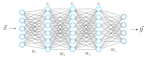
As before, we calculate the dot product between the input x and the first weight matrix W1, and apply an activation function to the resulting vector to obtain the first hidden vector h1. We now consider h1 the input for the upcoming third layer. We repeat the whole procedure from before until we obtain the final output y:
Loss Functions in Deep Learning
After we get the prediction of the neural network, we must compare this prediction vector to the actual ground truth label. We call the ground truth label vector y_hat.
While the vector y contains predictions that the neural network has computed during the forward propagation (which may, in fact, be very different from the actual values), the vector y_hat contains the actual values.
Mathematically, we can measure the difference between y and y_hat by defining a loss function, whose value depends on this difference.
An example of a general loss function is the quadratic loss:

The value of this loss function depends on the difference between y_hat and y. A higher difference means a higher loss value and a smaller difference means a smaller loss value.
Minimizing the loss function directly leads to more accurate predictions of the neural network, as the difference between the prediction and the label decreases.
Minimizing the loss function automatically causes the neural network model to make better predictions regardless of the exact characteristics of the task at hand. You only have to select the right loss function for the task.
Fortunately, there are only two loss functions that you should know about to solve almost any problem that you encounter in practice: the cross-entropy loss and the mean squared error (MSE) loss.
The Cross-Entropy Loss

Mean Squared Error Loss

Since the loss depends on the weight, we must find a certain set of weights for which the value of the loss function is as small as possible. The method of minimizing the loss function is achieved mathematically by a method called gradient descent.
Gradient Descent in Deep Learning
During gradient descent, we use the gradient of a loss function (the derivative, in other words) to improve the weights of a neural network.
To understand the basic concept of the gradient descent process, let’s consider a basic example of a neural network consisting of only one input and one output neuron connected by a weight value w.

This neural network receives an input x and outputs a prediction y. Let's say the initial weight value of this neural network is 5 and the input x is 2. Therefore the prediction y of this network has a value of 10, while the label y_hat might have a value of 6.

This means that the prediction is not accurate and we must use the gradient descent method to find a new weight value that causes the neural network to make the correct prediction. In the first step, we must choose a loss function for the task.
Let’s take the quadratic loss that I defined above and plot this function, which is basically just a quadratic function:
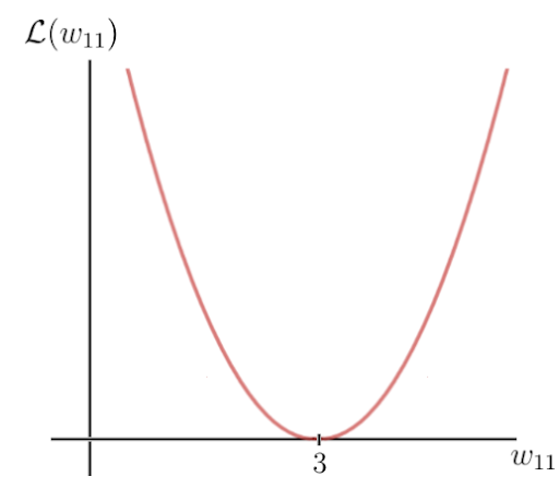
The y-axis is the loss value, which depends on the difference between the label and the prediction, and thus the network parameters — in this case, the one weight w. The x-axis represents the values for this weight.
As you can see, there is a certain weight w for which the loss function reaches a global minimum. This value is the optimal weight parameter that would cause the neural network to make the correct prediction (which is 6). In this case, the value for the optimal weight is 3:
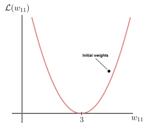
On the other hand, our initial weight is 5, which leads to a fairly high loss. The goal now is to repeatedly update the weight parameter until we reach the optimal value for that particular weight. This is the time when we need to use the gradient of the loss function.
Fortunately, in this case, the loss function is a function of one single variable, the weight w:

In the next step, we calculate the derivative of the loss function with respect to this parameter:

In the end, we get 8, which gives us the value of the slope or the tangent of the loss function for the corresponding point on the x-axis, at which point our initial weight lies.
This tangent points toward the highest rate of increase of the loss function and the corresponding weight parameters on the x-axis.
This means that we have just used the gradient of the loss function to find out which weight parameters would result in an even higher loss value. What we really want to know is the exact opposite. We can get what we want if we multiply the gradient by -1 and, in this way, obtain the opposite direction of the gradient.
This is how we get the direction of the loss function’s highest rate of decrease and the corresponding parameters on the x-axis that cause this decrease:
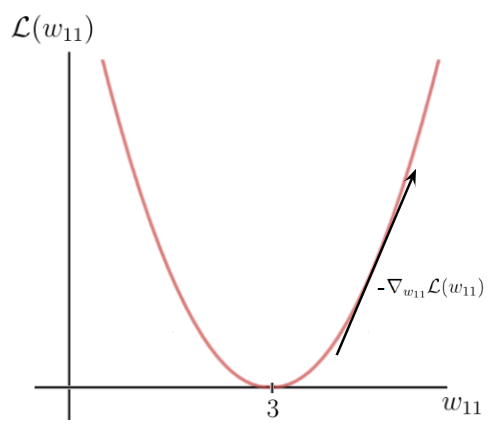
Finally, we perform one gradient descent step as an attempt to improve our weights. We use this negative gradient to update your current weight in the direction of the weights for which the value of the loss function decreases, according to the negative gradient:


The factor epsilon in this equation is a hyper-parameter called the learning rate. The learning rate determines how quickly or how slowly you want to update the parameters.
Please keep in mind that the learning rate is the factor with which we have to multiply the negative gradient and that the learning rate is usually quite small. In our case, the learning rate is 0.1.
As you can see, our weight w after the gradient descent is now 4.2 and closer to the optimal weight than it was before the gradient step.
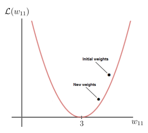
The value of the loss function for the new weight value is also smaller, which means that the neural network is now capable of making better predictions. You can do the calculation in your head and see that the new prediction is, in fact, closer to the label than before.
Each time we update the weights, we move down the negative gradient towards the optimal weights.
After each gradient descent step or weight update, the current weights of the network get closer and closer to the optimal weights until we eventually reach them. At that point, the neural network will be capable of making the predictions we want to make.
Frequently Asked Questions
What is deep learning?
Deep learning is a type of machine learning and artificial intelligence that uses neural network algorithms to analyze data and solve complex problems. Neural networks in deep learning are comprised of multiple layers of artificial nodes and neurons, which help process information.
What is the difference between machine learning and deep learning?
Machine learning is a type of artificial intelligence designed to learn from data on its own and adapt to new tasks without explicitly being programmed to.
Deep learning is a subset of machine learning and type of artificial intelligence that uses artificial neural networks to mimic the structure and problem-solving capabilities of the human brain.


