How Loss Functions Work in Neural Networks and Deep Learning

Before we discuss different kinds of loss functions used in deep learning, let’s talk about why we need loss functions in the first place. To do that, we first need to learn about what’s happening inside a neural network.

More From Artem OppermannArtificial Intelligence vs. Machine Learning vs. Deep Learning

Why Do We Need Loss Functions in Deep Learning?

There are two possible mathematical operations happening inside a neural network:

• Forward propagation
• Backpropagation with gradient descent

While forward propagation refers to the computational process of predicting an output for a given input vector x, backpropagation and gradient descent describe the process of improving the weights and biases of the network in order to make better predictions. Let’s look at this in practice. 

For a given input vector x the neural network predicts an output, which is generally called a prediction vector y.

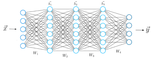
The equations describing the mathematics happening during the prediction vector’s computation looks like this:

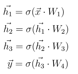
We must compute a dot-product between the input vector x and the weight matrix W1 that connects the first layer with the second. After that, we apply a non-linear activation function to the result of the dot-product. 

The prediction vector can represent a number of things depending on the task we want the network to do. For regression tasks, which are basically predictions of continuous variables (e.g. stock price, expected demand for products, etc.), the output vector y contains continuous numbers. 

Regardless of the task, we somehow have to measure how close our predictions are to the ground truth label.        

On the other hand, for classification tasks, such as customer segmentation or image classification, the output vector y represents probability scores between 0.0 and 1.0.

The value we want the neural network to predict is called a ground truth label, which is usually represented as y_hat. A predicted value y closer to the label suggests a better performance of the neural network.

Regardless of the task, we somehow have to measure how close our predictions are to the ground truth label.

This is where the concept of a loss function comes into play.

Mathematically, we can measure the difference (or error) between the prediction vector y and the label y_hat by defining a loss function whose value depends on this difference.

An example of a general loss function is the quadratic loss:

Since the prediction vector y(θ) is a function of the neural network’s weights (which we abbreviate to θ), the loss is also a function of the weights.

Since the loss depends on weights, we must find a certain set of weights for which the value of the loss function is as small as possible. We achieve this mathematically through a method called gradient descent.

The value of this loss function depends on the difference between the label y_hat and y. A higher difference means a higher loss value while (you guessed it) a smaller difference means a smaller loss value. Minimizing the loss function directly leads to more accurate predictions of the neural network as the difference between the prediction and the label decreases.

The neural network’s only objective is to minimize the loss function.

In fact, the neural network’s only objective is to minimize the loss function. This is because minimizing the loss function automatically causes the neural network model to make better predictions regardless of the exact characteristics of the task at hand.

A neural network solves tasks without being explicitly programmed with a task-specific rule. This is possible because the goal of minimizing the loss function is universal and doesn’t depend on the task or circumstances.

3 Key Types of Loss Functions in Neural Networks

That said, you still have to select the right loss function for the task at hand. Luckily there are only three loss functions you need to know to solve almost any problem.

1. Mean Squared Error Loss Function

Mean squared error (MSE) loss function is the sum of squared differences between the entries in the prediction vector y and the ground truth vector y_hat.

You divide the sum of squared differences by N, which corresponds to the length of the vectors. If the output y of your neural network is a vector with multiple entries then N is the number of the vector entries with y_i being one particular entry in the output vector.

The mean squared error loss function is the perfect loss function if you're dealing with a regression problem. That is, if you want your neural network to predict a continuous scalar value.

An example of a regression problem would be predictions of . . . 

• the number of products needed in a supply chain.

• future real estate prices under certain market conditions.

• a stock value.

Here is a code snippet where I've calculated MSE loss in Python:

import numpy as np

# The prediction vector of the neural network
y_pred=[0.6, 1.29, 1.99, 2.69, 3.4]

# The ground truth label
y_hat= [1, 1, 2, 2, 4]

# Mean squared error
MSE = np.sum(np.square(np.subtract(y_hat, y_pred)))/len(y_hat)

print(MSE) # The result is 0.21606

Learn More From Our ExpertsWhat Is Linear Regression?

2. Cross-Entropy Loss Function

Regression is only one of two areas where feedforward networks enjoy great popularity. The other area is classification.

In classification tasks, we deal with predictions of probabilities, which means the output of a neural network must be in a range between zero and one. A loss function that can measure the error between a predicted probability and the label which represents the actual class is called the cross-entropy loss function.

One important thing we need to discuss before continuing with the cross-entropy is what exactly the ground truth vector looks like in the case of a classification problem.

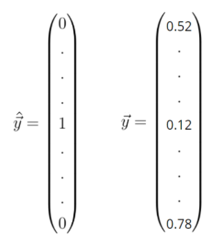
The label vector y_hat is one hot encoded which means the values in this vector can only take discrete values of either zero or one. The entries in this vector represent different classes. The values of these entries are zero, except for a single entry which is one. This entry tells us the class into which we want to classify the input feature vector x.

The prediction y, however, can take continuous values between zero and one.

Given the prediction vector y and the ground truth vector y_hat you can compute the cross-entropy loss between those two vectors as follows:

First, we need to sum up the products between the entries of the label vector y_hat and the logarithms of the entries of the predictions vector y. Then we must negate the sum to get a positive value of the loss function.

One interesting thing to consider is the plot of the cross-entropy loss function. In the following graph, you can see the value of the loss function (y-axis) vs. the predicted probability y_i. Here y_i takes values between zero and one.

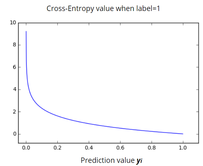
We can see clearly that the cross-entropy loss function grows exponentially for lower values of the predicted probability y_i. For y_i=0 the function becomes infinite, while for y_i=1 the neural network makes an accurate probability prediction and the loss value goes to zero.

Here’s another code snippet in Python where I’ve calculated the cross-entropy loss function:

import numpy as np

# The probabilities predicted by the neural network
y_pred = [0.1, 0.3, 0.4, 0.2]

# one-hot-encoded ground truth label
y_hat =[0, 1, 0, 0]

cross_entropy = - np.sum(np.log(y_pred)*y_hat)

print(cross_entropy) # The Result is 1.20

Read More From Our Machine Learning ExpertsMachine Learning for Beginners

3. Mean Absolute Percentage Error

Finally, we come to the Mean Absolute Percentage Error (MAPE) loss function. This loss function doesn’t get much attention in deep learning. For the most part, we use it to measure the performance of a neural network during demand forecasting tasks.

First thing first: what is demand forecasting?

Demand forecasting is the area of predictive analytics dedicated to predicting the expected demand for a good or service in the near future. For example:

• In retail, we can use demand forecasting models to determine the amount of a particular product that should be available and at what price.

• In industrial manufacturing, we can predict how much of each product should be produced, the amount of stock that should be available at various points in time, and when maintenance should be performed.

• In the travel and tourism industry, we can use demand forecasting models to assess optimal price points for flights and hotels, in light of available capacity, what price should be assigned (for hotels, flights), which destinations should be spotlighted, or, what types of packages should be advertised.

Although demand forecasting is also a regression task and the minimization of the MSE loss function is an adequate training goal, this type of loss function to measure the performance of the model during training isn’t suitable for demand forecasting.

Why is that?

Well, imagine the MSE loss function gives you a value of 100. Can you tell if this is generally a good result? No, because it depends on the situation. If the prediction y of the model is 1000 and the actual ground truth label y_hat is 1010, then the MSE loss of 100 would be in fact a very small error and the performance of the model would be quite good.

However in the case where the prediction would be five and the label is 15, you would have the same loss value of 100 but the relative deviation to the ground-truth value would be much higher than in the previous case.

This example shows the shortcoming of the mean squared error function as the loss function for the demand forecasting models. For this reason, I strongly recommend using mean absolute percentage error (MAPE).

The mean absolute percentage error, also known as mean absolute percentage deviation (MAPD) usually expresses accuracy as a percentage. We define it with the following equation:

In this equation, y_i is the predicted value and y_hat is the label. We divide the difference between y_i and y_hat by the actual value y_hat again. Finally, multiplying by 100 percent gives us the percentage error.

Applying this equation to the example above gives you a more meaningful understanding of the model’s performance. In the first case, the deviation from the ground truth label would be only one percent, while in the second case the deviation would be 66 percent:

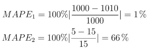
We see that the performance of these two models is very different. Meanwhile, the MSE loss function would indicate that the performance of both models is the same.

The following Python code snipped shows how we can calculate MAPE:

ximport numpy as np

# The prediction vector of the neural network
y_pred=[0.6, 1.29, 1.99, 2.69, 3.4]

# The ground truth label
y_hat= [1, 1, 2, 2, 4]

MAPE = (100.0/len(y_hat))*np.sum(np.abs(y_pred-y_hat)/y_hat)

print(MAPE) # The result is mean percentage error of 23.79%

Best Practices for Loss Functions and Neural Networks

When you’re working with loss functions, just remember these key principles:

• A loss function measures how good a neural network model is in performing a certain task, which in most cases is regression or classification.

• We must minimize the value of the loss function during the backpropagation step in order to make the neural network better.

• We only use the cross-entropy loss function in classification tasks when we want the neural network to predict probabilities.

• For regression tasks, when we want the network to predict continuous numbers, we must use the mean squared error loss function.

• We use mean absolute percentage error loss function during demand forecasting to keep an eye on the performance of the network during training time.