How to Get Started With Regression Trees

Regression trees, a variant of decision trees, aim to predict outcomes we would consider real numbers such as the optimal prescription dosage, the cost of gas next year or the number of expected Covid-19 cases this winter. At their core, decision tree models are nested if-else conditions. We can think of this model as a tree because regression models attempt to determine the relationship between one dependent variable and a series of independent variables that split off from the initial data set. 

In this article, we’ll walk through an overview of the decision tree algorithm used for regression task setting. Let’s jump in.

Basics of Decision Tree

In this section, we’ll work on a pollution data set, which consists of seven explanatory variables; the target is to understand not only the pollution level, but what’s causing the pollution. First we’ll make a skeleton model using the R tree module and analyze the results.

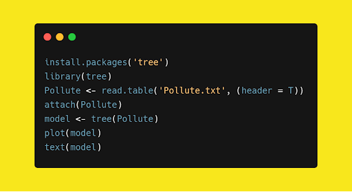
In this code, we’ve imported a tree module in CRAN packages (Comprehensive R Archive Network) because it has a decision tree functionality. The result of the above code is as follows:

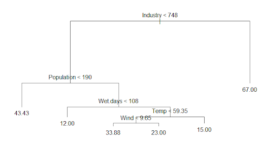
As you can see, this decision tree is an upside-down schema. Usually a decision tree takes a sample of variables available (or takes all available variables at once) for splitting. A split is determined on the basis of criteria like Gini Index or Entropy with respect to variables. 

Subspace is a p-dimensional space of p explanatory variables/features unto which the regression task is to be determined.

Now let’s look at the root and internal nodes of our tree:

• Industry < 748
• Population < 190
• Wet Days < 108
• Temp < 59.35
• Wind < 9.65  

As you can see, each terminal node has branches, which might terminate or split, giving us our tree shape. For example, terminal splitting occurs based on Gini Index or Entropy.

For any test data, if Population < 190 then the tree’s output is 43.43. This output is based on the mean observation in the training set which splits that particular region.

More Exercises Using RBaffled by Covariance vs. Correlation? You’re Not Alone.

The Math Behind Regression Trees

Above, we used R to make a decision tree of our pollution use-case but it’s paramount to know and understand what’s actually behind the code. We need to understand why our algorithm decided to split variables, split points and what topology the tree should have. There are two steps involved:

1. We divide the predictor space set of possible feature variables into distinct and non-overlapping regions.

2. For every observation that falls into a region, we predict which is the mean response in the training set.

In theory, we can make any shape, but the algorithm chooses to divide the space using high-dimensional rectangles or boxes that will make it easy to interpret the data. The goal is to find boxes which minimize the RSS (residual sum of squares).

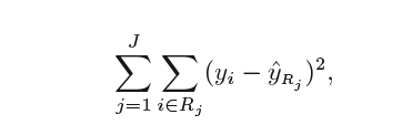
It is computationally infeasible to consider every possible partition of feature space into j boxes. To overcome this limitation, we go for a top-down, greedy approach known as recursive binary splitting. The approach is top-down as it starts at the top of the tree (where all observations fall into a single region) and successively splits the predictor space into two new branches. We call this approach greedy because, at each step, the algorithm chooses the best split at that particular region without consideration of the next steps.

In order to perform recursive binary splitting, we select the predictor and the cut point that leads to the greatest reduction in RSS.

We seek the value of j and s that minimize the equation.

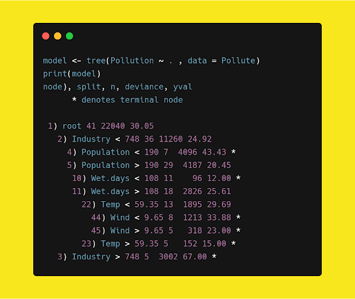
In this code, we see the detailed description of the tree above and how the deviance (or RSS) reduces with each split.

More From Our Data Science Experts4 Types of Projects You Need in Your Data Science Portfolio

Decision Tree Pruning: Cost Complexity Pruning

The process described above is overly optimistic about training data. In other words, the algorithm can overfit the data and perform poorly on test set performance. The overfit model ascertains high variance. On the other hand, a smaller tree with fewer splits might lead to lower variance with better interpretation but with a little higher bias. So what do you do? 

One strategy is to split the nodes if they decrease in RSS. This strategy works sometimes but not always. Tree size is a tuning parameter governing the model’s complexity and the optimal tree size should be attuned to the data itself. To overcome the danger of overfitting your model, we apply the cost complexity pruning algorithm.

The preferred strategy is to grow a large tree and stop the splitting process only when you reach some minimum node size (usually five). We define a subtree T that we can obtain by pruning, (i.e. collapsing the number of internal nodes). We index the terminal nodes by m, with node m representing the region Rm. Let |T| denote the number of terminal nodes in T.

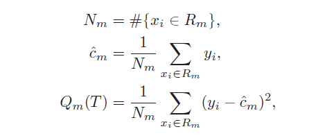
The tuning parameter governs the tradeoffs between tree size and its quality of fit. Large values of alpha result in smaller trees (and vice versa). This process is analogous to the procedure in ridge regression, where an increase in the value of tuning parameters will decrease the weights of coefficients. Estimation of alpha is achieved by five- or ten-fold cross-validation. 

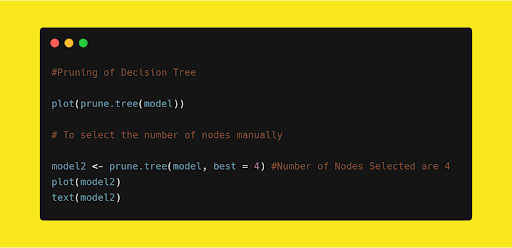
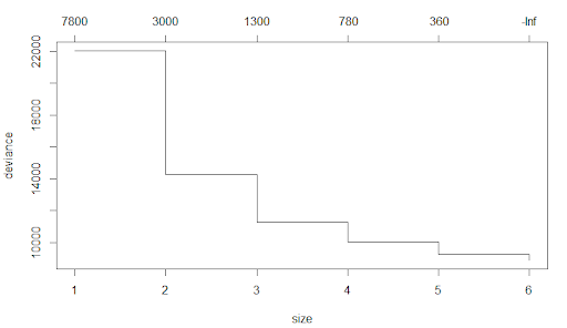
In the tree module, there is a method called prune.tree which gives a graph on the number of nodes versus deviance based on the cost complexity pruning. We can even manually select the nodes based on the graph.

Frequently Asked Questions