This is the first article of the multi-part series on self learning AI-Agents or — to put it more precisely — deep reinforcement learning. The aim of the series isn’t just to give you an overview but to provide you with a more in-depth exploration of the theory, mathematics and implementation behind the most popular and effective methods of deep reinforcement learning.
Deep reinforcement learning is on the rise. No other sub-field of deep learning has been more widely discussed in recent years by researchers, but also in the general media.
What Is Deep Reinforcement Learning?
Most outstanding achievements in deep learning are due to deep reinforcement learning from Google’s Alpha Go that beat the world’s best human chess player in the board game Go (an achievement assumed impossible a couple years earlier). The chess player lost to DeepMind’s AI agents that teach themselves to walk, run and overcome obstacles (see below).


Since 2014, other AI agents exceed humans in playing old school Atari games such as Breakout.

The most amazing thing about all of these examples is the fact that no humans programmed or explicitly taught these AI agents. The agents themselves learned by the power of deep and reinforcement learning.
So how does that work? I’ll begin demonstrating the necessary mathematical foundation to tackle the most promising areas in this sub-field of AI.
Deep Reinforcement Learning in a Nutshell
We can summarize deep reinforcement learning as building an algorithm (or an AI agent) that learns directly from its interaction with an environment (figure 5). The environment may be the real world, a computer game, a simulation or even a board game, like Go or chess. Like a human, the AI agent learns from consequences of its actions, rather than by being taught explicitly by a programmer. In other words, you might say these algorithms learn the hard way.

In deep reinforcement learning a neural network represents the AI agent. The neural network interacts directly with its environment. The network observes the current state of the environment and decides which action to take (e.g. move left, right, etc.) based on the current state and its past experiences. Based on the action the AI agent takes, it may receive a reward or consequence. The reward or consequence is merely a scalar. The negative consequence (e.g. -5) occurs if the agent performs poorly and the positive reward (e.g. +5) occurs if the agent performs well.
The quality of the action correlates directly to the quantity of the reward and is predictive of how likely the agent is to solve the problem (e.g. learning how to walk). In other words, the objective of an agent is to learn to take actions in any given circumstances that maximizes the accumulated reward over time.
Markov Decision Process
A Markov decision Process (MDP), a discrete time stochastic control process, is the best approach we have so far to model the complex environment of an AI agent. Every problem the agent aims to solve can be considered as a sequence of states: S1, S2, S3 ... Sn (a state may be, for example, a Go or chess board configuration). The agent takes actions and moves from one state to another. In what follows, I’ll show you the mathematics that determine which action the agent must take in any given situation.
Markov Processes
A Markov process (or Markov chain) is a stochastic model describing a sequence of possible states in which the current state depends on only the previous state. This is also called the Markov property (equation 1). For reinforcement learning it means the next state of an AI agent only depends on the last state and not all the previous states before.

A Markov process is stochastic, which means the transition from the current state s to the next state s’ can only happen with a certain probability Pss’ (equation 2). In a Markov process an agent that’s told to go left would go left only with a certain probability of, let’s say, 0.998. With such a small probability, where the agent will ultimately end up depends upon the environment — for example, the chess board and arrangement of pieces on it.

We can consider Pss’ can an entry in a state transition matrix P that defines transition probabilities from all states s to all successor states s’ (equation 3).

Remember: A Markov process is a tuple <S, P>. S is a (finite) set of states. P is a state transition probability matrix.
Markov Reward Process
A Markov reward process is also a tuple <S, P, R>. Here R is the reward the agent expects to receive in the state s (equation 4). The AI agent is motivated by the fact that, to achieve a certain goal (e.g. winning a chess game), certain states (game configurations) are more promising than others in terms of strategy and potential to win the game.

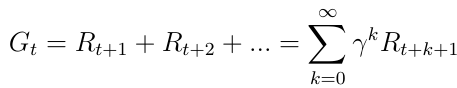
The primary topic of interest is the total reward Gt (equation 5), which is the expected accumulated reward the agent will receive across the sequence of all states. The discount factor γ ∈ [0, 1] weighs every reward. We find discounting rewards mathematically convenient since doing so avoids infinite returns in cyclic Markov processes. Besides, the discount factor means that, the more we consider the future, the less important the rewards become than immediate gratification, because the future is often uncertain. For example, if the reward is financial, immediate rewards may earn more interest than delayed rewards.
Value Function
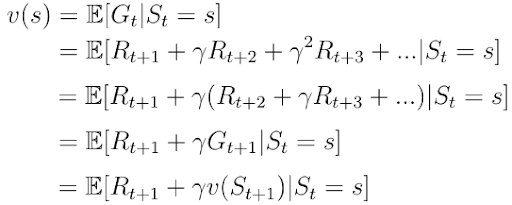
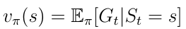
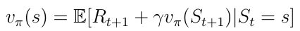
Another important concept is the one of the value function v(s). The value function maps a value to each state s. The value of a state s is defined as the expected total reward the AI agent will receive if it starts its progress in the state s (equation 6).

The value function can be decomposed into two parts:
-
The immediate reward
R(t+1)the agent receives being in states. -
The discounted value
v(s(t+1))of the next state after the states.
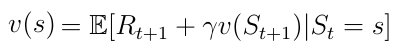
Bellman Equation
Bellman Equation for Markov Reward Processes
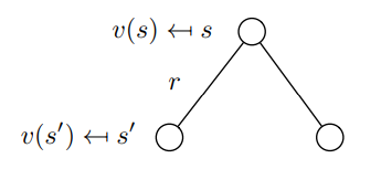
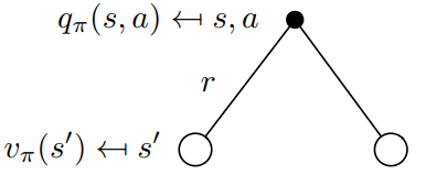
We also know the decomposed value function (equation 8) as the Bellman equation for Markov reward processes. We visualize this function using a node graph (figure 6). Starting in state s leads to the value v(s). Being in the state s we have a certain probability Pss’ to end up in the next state s’. In this particular case we have two possible next states. To obtain the value v(s) we must sum up the values v(s’) of the possible next states weighted by the probabilities Pss’ and add the immediate reward from being in state s. This yields equation nine, which is nothing more than equation eight if we were to execute the expectation operator E in the equation.

Markov Decision Process vs. Markov Reward Process
A Markov Decision Process is a Markov Reward Process with decisions. We can describe a Markov decision process with a set of tuples <S,A,P, R>. In this instance, A is a finite set of possible actions the agent can take in the state s. Thus, the immediate reward from being in state s now also depends on the action a the agent takes in this state (equation 10).

Policies
Let’s look at how the agent decides which action it must take in a particular state. The policy π determines the action (equation 11). Mathematically speaking, a policy is a distribution over all actions given a state s. The policy determines the mapping from a state s to the action the agent must take.

Put another way, we can describe the policy π as the agent’s strategy to select certain actions depending on the current state s.
The policy leads to a new definition of the state-value function v(s) (equation 12) which we define now as the expected return starting from state s, and then following a policy π.
Action-Value Function
Another important function to learn is the action-value function q(s,a) (equation 13), or the expected return we obtain by starting in state s, taking action a and then following a policy π. Notice that a state s, q(s,a) can take several values since there are several actions the agent can take in a state s.
A neural network calculates Q(s,a). Given a state s as input, the network calculates the quality for each possible action in this state as a scalar (figure 7). Higher quality means a better action with regards to the given objective.
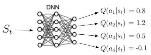
Remember: Action-value function tells us how good it is to take a particular action in a particular state.

Previously, the state-value function v(s) could be decomposed into the following form:
We can now apply the same decomposition to the action-value function:

At this point, let's discuss how v(s) and q(s,a) relate to each other. Again, we can visualize the relationship between these functions as:
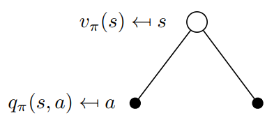
In this example, being in the state s allows us to take two possible actions a. By definition, taking a particular action in a particular state gives us the action-value q(s,a). The value function v(s) is the sum of possible q(s,a) weighted by the probability (which is none other than the policy π) of taking an action in the state s (equation 16).

Now let's consider the opposite case in figure nine, below. The root of the binary tree is now a state in which we choose to take a particular action a. Remember that the Markov processes are stochastic. Taking an action does not mean that you will end up where you want to be with 100 percent certainty. Strictly speaking, you must consider probabilities to end up in other states after taking the action.
In this particular case, after taking action a you can end up in two different next states s’:
To obtain the action-value you must take the discounted state-values weighted by the probabilities Pss’ to end up in all possible states (in this case only two) and add the immediate reward:
Now that we know the relation between those functions we can insert v(s) from equation 16 into q(s,a) from equation 17. We obtain equation 18 and notice there’s a recursive relationship between the current q(s,a) and the next action-value q(s’,a’).
We can visualize this recursive relationship in another binary tree (figure 10). We begin with q(s,a), end up in the next state s’ with a certain probability Pss’. From there we can take an action a’ with the probability π and we end with the action-value q(s’,a’). To obtain q(s,a) we must go up in the tree and integrate over all probabilities as you can see in equation 18.

Optimal Policy
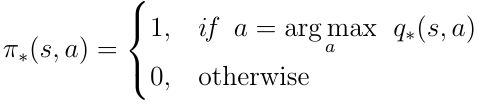
The most important topic of interest in deep reinforcement learning is finding the optimal action-value function q*. Finding q* means the agent knows exactly the quality of an action in any given state. Furthermore, the agent can decide which action it must take based on the quality.
Let's define what q* means. The best possible action-value function is the one that follows the policy that maximizes the action-values:

To find the best possible policy we must maximize over q(s, a). Maximization means we select only the action a from all possible actions for which q(s,a) has the highest value. This yields the following definition for the optimal policy π:
Bellman Optimality Equation
We can insert the condition for the optimal policy into equation 18, thus providing us with the Bellman optimality equation:
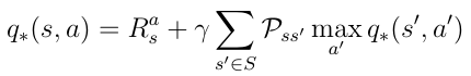
If the AI agent can solve this equation then it basically means it’s solved the problem in the given environment. The agent knows in any given state or situation the quality of any possible action with regards to the objective and can behave accordingly.
Solving the Bellman optimality equation will be the topic of upcoming articles in this series. In part two, I’ll demonstrate the first technique to solve the equation called Deep Q-learning.
Frequently Asked Questions
How do AI agents learn through reinforcement?
Agents observe the current state, choose actions and receive rewards or penalties. Over time, they learn which actions lead to better outcomes.
What is a Markov decision process (MDP)?
An MDP is a mathematical framework that models decision-making as a sequence of states, actions and rewards, assuming future states depend only on the current state.
How is a reward calculated in reinforcement learning?
Rewards are scalar values that reflect how good or bad an action was. The goal is to maximize the total accumulated reward over time.