How Does Backpropagation in a Neural Network Work?

Ever since nonlinear functions that work recursively (i.e., artificial neural networks) were introduced to the world of machine learning, applications of it have been booming. In this context, proper training of a neural network is the most important aspect of making a reliable model. This training is usually associated with the term backpropagation, which is a vague concept for most people getting into deep learning. Most people in the industry don’t even know how it works — they just know it does.

What Is Backpropagation?

Backpropagation is the essence of neural net training. It is the practice of fine-tuning the weights of a neural net based on the error rate (i.e. loss) obtained in the previous epoch (i.e. iteration.) Proper tuning of the weights ensures lower error rates, making the model reliable by increasing its generalization.

So how does this process with vast simultaneous mini-executions work? Let’s explore some examples.

In order to make this example as useful as possible, we’re just going to touch on related concepts like loss functions, optimization functions, etc., without explaining them, as these topics require their own articles.

Advantages of Using the Backpropagation Algorithm in Neural Networks

Before getting into the details of backpropagation in neural networks, let’s review the importance of this algorithm. Besides improving a neural network, below are a few other reasons why backpropagation is a useful approach: 

• No previous knowledge of a neural network is needed, making it easy to implement. 
• It’s straightforward to program since there are no other parameters besides the inputs.
• It doesn’t need to learn the features of a function, speeding up the process. 
• The model is flexible because of its simplicity and applicable to many scenarios. 

Limitations of Using the Backpropagation Algorithm in Neural Networks

That said, backpropagation is not a blanket solution for any situation involving neural networks. Some of the potential limitations of this model include:

• Training data can impact the performance of the model, so high-quality data is essential. 
• Noisy data can also affect backpropagation, potentially tainting its results.  
• It can take a while to train backpropagation models and get them up to speed.  
• Backpropagation requires a matrix-based approach, which can lead to other issues.

Although backpropagation has its flaws, it’s still an effective model for testing and refining the performance of neural networks. Now that we understand the pros and cons of this algorithm, let’s take a deeper look at the ins and outs of backpropagation in neural networks.     

How to Set the Model Components for a Backpropagation Neural Network

Imagine that we have a deep neural network that we need to train. The purpose of training is to build a model that performs the exclusive OR (XOR) functionality with two inputs and three hidden units, such that the training set (truth table) looks something like the following:

X1 | X2 | Y
0  | 0  | 0
0  | 1  | 1
1  | 0  | 1 
1  | 1  | 0

We also need an activation function that determines the activation value at every node in the neural net. For simplicity, let’s choose an identity activation function:f(a) = a

We also need a hypothesis function that determines the input to the activation function. This function is going to be the ever-famous:

h(X) = W0.X0 + W1.X1 + W2.X2

            or

h(X) = sigma(W.X) for all (W, X)

Let’s also make the loss function the usual cost function of logistic regression. It looks a bit complicated, but it’s actually fairly simple:

We’re going to use the batch gradient descent optimization function to determine in what direction we should adjust the weights to get a lower loss than our current one. Finally, we’ll set the learning rate to 0.1 and all the weights will be initialized to one.

More on Neural NetworksTransformer Neural Networks: A Step-by-Step Breakdown

Building a Neural Network

Let’s finally draw a diagram of our long-awaited neural net. It should look something like this:

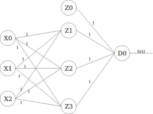
The leftmost layer is the input layer, which takes X0 as the bias term of value one, and X1 and X2 as input features. The layer in the middle is the first hidden layer, which also takes a bias term Z0 value of one. Finally, the output layer has only one output unit D0 whose activation value is the actual output of the model (i.e. h(x).)

How Forward Propagation Works

It is now the time to feed-forward the information from one layer to the next. This goes through two steps that happen at every node/unit in the network:

1. Getting the weighted sum of inputs of a particular unit using the h(x) function we defined earlier.
2. Plugging the value we get from step one into the activation function, we have (f(a)=a, in this example) and using the activation value we get the output of the activation function as the input feature for the connected nodes in the next layer.

Units X0, X1, X2 and Z0 do not have any units connected to them providing inputs. Therefore, the steps mentioned above do not occur in those nodes. However, for the rest of the nodes/units, this is how it all happens throughout the neural net for the first input sample in the training set:

Unit Z1:
       h(x) = W0.X0 + W1.X1 + W2.X2
            = 1 . 1 + 1 . 0 + 1 . 0
            = 1 = a

       z = f(a) = a   =>   z = f(1) = 1

Same goes for the remaining units:

Unit Z2:
       h(x) = W0.X0 + W1.X1 + W2.X2
            = 1 . 1 + 1 . 0 + 1 . 0
            = 1 = a
       z = f(a) = a   =>   z = f(1) = 1

Unit Z3:
       h(x) = W0.X0 + W1.X1 + W2.X2
            = 1 . 1 + 1 . 0 + 1 . 0
            = 1 = a
       z = f(a) = a   =>   z = f(1) = 1

Unit D0:
       h(x) = W0.Z0 + W1.Z1 + W2.Z2 + W3.Z3
            = 1 . 1 + 1 . 1 + 1 . 1 + 1 . 1
            = 4 = a
       z = f(a) = a   =>   z = f(4) = 4

As we mentioned earlier, the activation value (z) of the final unit (D0) is that of the whole model. Therefore, our model predicted an output of one for the set of inputs {0, 0}. Calculating the loss/cost of the current iteration would follow:

Loss = actual_y - predicted_y
    =    0     -     4
    =    -4

The actual_y value comes from the training set, while the predicted_y value is what our model yielded. So the cost at this iteration is equal to -4.

When Do You Use Backpropagation in Neural Networks?

According to our example, we now have a model that does not give accurate predictions. It gave us the value four instead of one and that is attributed to the fact that its weights have not been tuned yet. They’re all equal to one. We also have the loss, which is equal to -4. Backpropagation is all about feeding this loss backward in such a way that we can fine-tune the weights based on this. The optimization function, gradient descent in our example, will help us find the weights that will hopefully yield a smaller loss in the next iteration. So, let’s get to it.

If feeding forward happened using the following functions: f(a) = a

Then feeding backward will happen through the partial derivatives of those functions. There is no need to go through the equation to arrive at these derivatives. All we need to know is that the above functions will follow:

f'(a) = 1

J'(w) = Z . delta

Z is just the z value we obtained from the activation function calculations in the feed-forward step, while delta is the loss of the unit in the layer.

I know it’s a lot of information to absorb in one sitting, but I suggest you take your time to really understand what is going on at each step before going further.

How to Calculate Deltas in Backpropagation Neural Networks

Now we need to find the loss at every unit/node in the neural net. Why is that? Well, think about it this way: Every loss the deep learning model arrives at is actually the mess that was caused by all the nodes accumulated into one number. Therefore, we need to find out which node is responsible for the most loss in every layer, so that we can penalize it by giving it a smaller weight value, and thus lessening the total loss of the model.

Calculating the delta for every unit can be problematic. However, thanks to computer scientist and founder of DeepLearning, Andrew Ng, we now have a shortcut formula for the whole thing:

delta_0 = w . delta_1 . f'(z)

Where values delta_0, w and f’(z) are those of the same unit’s, while delta_1 is the loss of the unit on the other side of the weighted link. For example:

In order to get the loss of a node (e.g. Z0), we multiply the value of its corresponding f’(z) by the loss of the node it is connected to in the next layer (delta_1), by the weight of the link connecting both nodes.

This is how backpropagation works. We do the delta calculation step at every unit, backpropagating the loss into the neural net, and find out what loss every node/unit is responsible for.

Let’s calculate those deltas.

delta_D0 = total_loss = -4

delta_Z0 = W . delta_D0 . f'(Z0) = 1 . (-4) . 1 = -4
delta_Z1 = W . delta_D0 . f'(Z1) = 1 . (-4) . 1 = -4
delta_Z2 = W . delta_D0 . f'(Z2) = 1 . (-4) . 1 = -4
delta_Z3 = W . delta_D0 . f'(Z3) = 1 . (-4) . 1 = -4

There are a few things to note here:

• The loss of the final unit (i.e. D0) is equal to the loss of the whole model. This is because it is the output unit, and its loss is the accumulated loss of all the units together.
• The function f’(z)will always give the value one, no matter what the input (i.e. z) is equal to. This is because the partial derivative, as we said earlier, follows: f’(a) = 1
• The input nodes/units (X0, X1 and X2) don’t have delta values, as there is nothing those nodes control in the neural net. They are only there as a link between the data set and the neural net. This is why the whole layer is usually not included in the layer count.

More on AIHow to Get Started With Regression Trees

Updating the Weights in Backpropagation for a Neural Network

All that’s left is to update all the weights we have in the neural net. This follows the batch gradient descent formula:

W := W - alpha . J'(W)

Where W is the weight at hand, alpha is the learning rate (i.e. 0.1 in our example) and J’(W) is the partial derivative of the cost function J(W) with respect to W. Again, there’s no need for us to get into the math. Therefore, let’s use Mr. Andrew Ng’s partial derivative of the function:

J'(W) = Z . delta

Where Z is the Z value obtained through forward propagation, and delta is the loss at the unit on the other end of the weighted link:

Now we use the batch gradient descent weight update on all the weights, utilizing our partial derivative values that we obtain at every step. It is worth emphasizing that the Z values of the input nodes (X0, X1, and X2) are equal to one, zero, zero, respectively. The one is the value of the bias unit, while the zeroes are actually the feature input values coming from the data set. There is no particular order to updating the weights. You can update them in any order you want, as long as you don’t make the mistake of updating any weight twice in the same iteration.

In order to calculate the new weights, let’s give the links in our neural nets names:

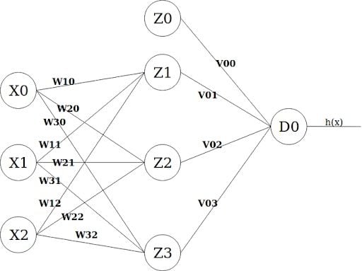
New weight calculations will happen as follows:

W10 := W10 - alpha . Z_X0 . delta_Z1
     =  1  -  0.1  .  1   .   (-4)   = 1.4
W20 := W20 - alpha . Z_X0 . delta_Z2
     =  1  -  0.1  .  1   .   (-4)   = 1.4
.       .      .      .        .
.       .      .      .        .
.       .      .      .        .
W30 := 1.4
W11 := 1.4
W21 := 1.4
W31 := 1.4
W12 := 1.4
W22 := 1.4
W32 := 1.4
V00 := V00 - alpha . Z_Z0 . delta_D0
     =  1  -  0.1  .  1   .   (-4)   = 1.4
V01 := 1.4
V02 := 1.4
V03 := 1.4

The model is not trained properly yet, as we only back-propagated through one sample from the training set. Doing everything all over again for all the samples will yield a model with better accuracy as we go, with the aim of getting closer to the minimum loss/cost at every step.

It might not make sense that all the weights have the same value again. However, training the model on different samples over and over again will result in nodes having different weights based on their contributions to the total loss.

The theory behind machine learning can be really difficult to grasp if it isn’t tackled the right way. One example of this would be backpropagation, whose effectiveness is visible in most real-world deep learning applications, but it’s never examined. Backpropagation is just a way of propagating the total loss back into the neural network to know how much of the loss every node is responsible for, and subsequently updating the weights in a way that minimizes the loss by giving the nodes with higher error rates lower weights, and vice versa.

Best Practices for Optimizing Backpropagation

Backpropagation in a neural network is designed to be a seamless process, but there are still some best practices you can follow to make sure a backpropagation algorithm is operating at peak performance. 

Select a Training Method

The pace of the training process depends on the method you choose. Going with a stochastic gradient descent speeds up the training, but the actual fine-tuning of the backpropagation algorithm can be tedious. On the other hand, batch gradient descent is easier to perform, but the overall learning process takes longer. For these reasons, the stochastic approach is preferred, but it’s important to pick a training method that best fits your circumstances. 

Provide Plenty of Data

Feeding a backpropagation algorithm lots of data is key to reducing the amount and types of errors it produces during each iteration. The size of your data set can vary, depending on the learning rate of your algorithm. In general, though, it’s better to include larger data sets since models can gain broader experiences and lessen their mistakes in the future.  

Clean All Data 

Backpropagation training is much smoother when the training data is of the highest quality, so clean your data before feeding it to your algorithm. This means normalizing the input values, which involves checking that the mean of the data is zero and the data set has a standard deviation of one. A backpropagation algorithm can then more easily analyze the data, leading to faster and more accurate results.  

Consider the Impacts of Learning Rate

Deciding on the learning rate for training a backpropagation model depends on the size of the data set, the type of problem and other factors. That said, a higher learning rate can lead to faster results, but not the optimal performance. A lower learning rate produces slower results, but can lead to a better outcome in the end. You’ll want to consider which learning rate best applies to your situation, so you don’t under- or overshoot your desired outcome. 

Test the Model With Different Examples

To get a sense of how well a backpropagation model performs, it helps to test the algorithm with data not used during the training period. Compiling diverse data also exposes the model to different situations and tests how well it can adapt to a range of scenarios. You can then make more informed adjustments to enhance the algorithm’s learning process.

Frequently Asked Questions