Fully Connected Layer vs. Convolutional Layer: Explained

The design of a neural network can be a difficult thing to get your head around at first. Designing a neural network involves choosing many design features like the input and output sizes of each layer, where and when to apply batch normalization layers and dropout layers, what activation functions to use, and more. I want to discuss what is really going on behind fully connected layers and convolutions, and how the output size of convolutional layers can be calculated.

Deep learning is a field of research that has skyrocketed in the past few years with the increase in computational power and advancements in the architecture of models. Two kinds of networks you’ll often encounter when reading about deep learning are fully connected neural networks (FCNN), and convolutional neural networks (CNNs). These two are the basis of deep learning architectures, and almost all other deep learning neural networks stem from these. I’ll first explain how fully connected layers work, then convolutional layers before finally going over an example of a CNN.

What Is a Fully Connected Layer?

Neural networks are a set of dependent non-linear functions. Each individual function consists of a neuron (or a perceptron). In fully connected layers, the neuron applies a linear transformation to the input vector through a weights matrix. A non-linear transformation is then applied to the product through a non-linear activation function f.

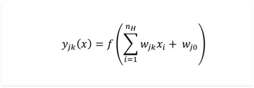
Here, we are taking the dot product between the weights matrix W and the input vector x. The bias term (W0) can be added inside the non-linear function. I will ignore it for the rest of the article as it doesn’t affect the output sizes or decision-making and is just another weight.

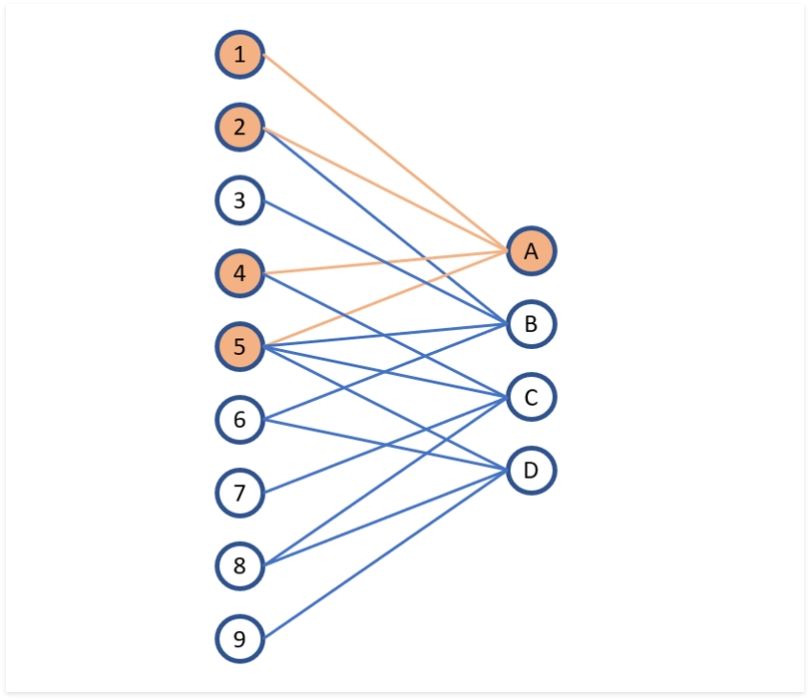
If we take a layer in a fully connected neural network with an input size of nine and an output size of four, the operation can be visualized as follows:

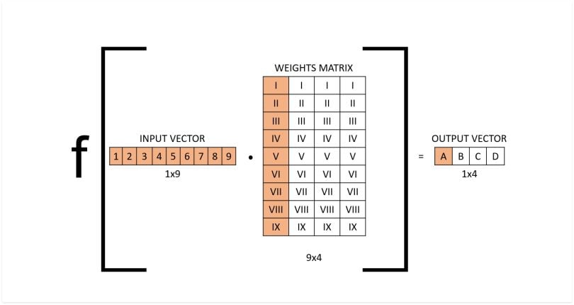
The activation function “f” wraps the dot product between the input of the layer and the weights matrix of that layer. Note that the columns in the weights matrix would all have different numbers and would be optimized as the model is trained.

The input is a 1x9 vector, the weights matrix is a 9x4 matrix. By taking the dot product and applying the non-linear transformation with the activation function we get the output vector (1x4).

You can also visualize this layer the following way:

Why Is It Called a Fully Connected Layer?

The image above shows why we call these kinds of layers “fully connected” or sometimes “densely connected.” All possible connections layer-to-layer are present, meaning every input of the input vector influences every output of the output vector. However, not all weights affect all outputs. Look at the lines between each node above. The orange lines represent the first neuron (or perceptron) of the layer. The weights of this neuron only affect output A, and do not have an effect on outputs B, C or D.

More on Machine Learning: Artificial Intelligence vs. Machine Learning vs. Deep Learning: What’s the Differenc

Convolutional Layer Explained

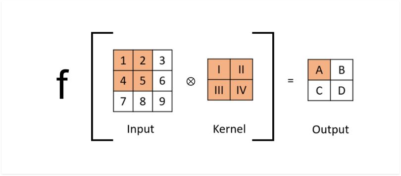
A convolution is effectively a sliding dot product, where the kernel shifts along the input matrix, and we take the dot product between the two as if they were vectors. Below is the vector form of the convolution shown above. You can see why taking the dot product between the fields in orange outputs a scalar (1x4 • 4x1 = 1x1).

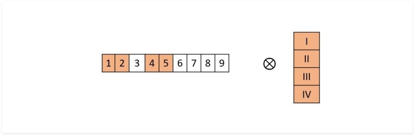
 Once again, we can visualize this convolutional layer as follows:

Convolutions are not densely connected; not all input nodes affect all output nodes. This gives convolutional layers more flexibility in learning. Moreover, the number of weights per layer is a lot smaller, which helps with high-dimensional inputs such as image data. These advantages are what give CNNs their well-known characteristic of learning features in the data, such as shapes and textures in image data.

How to Work With Fully Connected Layers and Convolutional Neural Networks

In FC layers, the output size of the layer can be specified very simply by choosing the number of columns in the weights matrix. The same cannot be said for convolutional layers. Convolutions have a lot of parameters that can be changed to adapt the output size of the operation.

In this explanation of convolutions, you’ll see all the variations of convolutions, such as convolutions with and without padding, strides, transposed convolutions and more. It’s a useful visual interpretation of a convolution. I still refer back to it often.

How to Calculate the Output Size of a Convolutional Layer

To determine the output size of the convolution, the following equation can be applied:

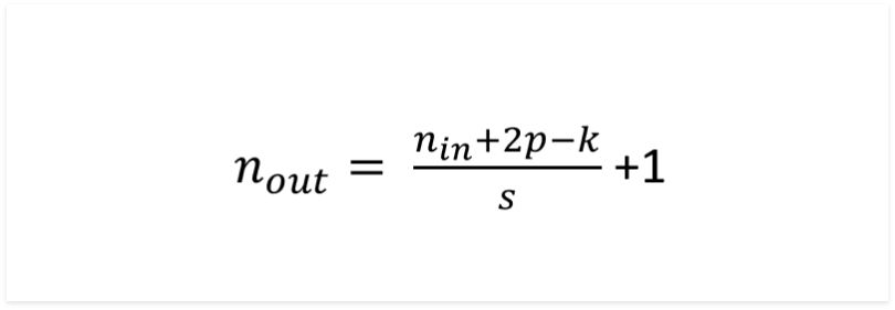
The output size is equal to the input size plus two times the padding minus the kernel size over the stride plus one. Most of the time we are dealing with square matrices, so this number will be the same for rows and columns. If the fraction does not result in an integer, we round up. It’s important to understand the equation. Dividing by the stride makes sense for the reason that when we skip over operations, we are dividing the output size by that number. Two times the padding comes from the fact that the padding is added on both sides of the matrix, and therefore is added twice.

How to Find the Transposed Convolutional Size

From the equation above, the output will always be equal to or smaller than the output, unless we add a lot of padding. However, adding too much padding to increase the dimensionality would result in greater difficulty in learning, as the inputs to each layer would be very sparse. To combat this, transposed convolutions are used to increase the size of the input. Example applications can be found in convolutional variational autoencoders (VAEs) or generative adversarial networks (GANs).

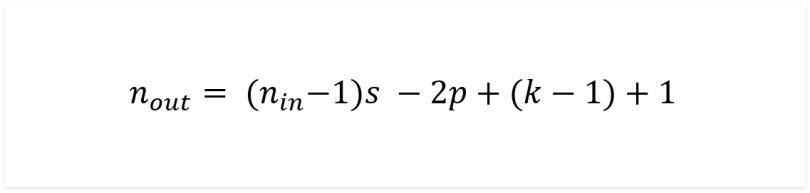
The above equation can be used to calculate the output size of a transposed convolutional layer.

With these two equations, you are now ready to design a convolutional neural network. Let’s take a look at the design of a GAN and understand it using the equations above.

More on Machine Learning: How Artificial Intelligence and Machine Learning Will Reshape Enterprise Technology

GAN Example

Here, I’ll go through the architecture of a GAN that uses convolutional and transposed convolutional layers. You’ll see why the equations above are so important and why you cannot design a CNN without them.

Let’s first take a look at the discriminator:

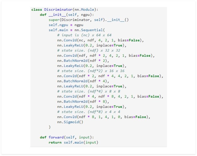
The input size to the discriminator is a 3x64x64 image, the output size is a binary 1x1 scalar. We are heavily reducing the dimensionality, therefore standard convolutional layers are ideal for this application.

Note that between each convolutional layer (denoted as Conv2d in PyTorch) the activation function is specified (in this case LeakyReLU), and batch normalization is applied.

Convolutional Layer in Discriminator

nn.Conv2d(nc, ndf, k = 4, s = 2, p = 1, bias=False)

The first convolutional layer applies the number of dimensions of the feature maps (ndf) convolutions to each of the three layers of the input. Image data often has three layers, one each for red, green and blue (RGB images). We can apply a number of convolutions to each of the layers to increase the dimensionality.

The first convolution applied has a kernel size of four, a stride of two and a padding of one. Plugging this into the equation gives:

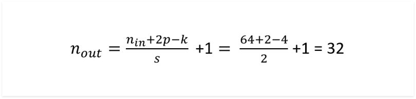
So the output is a 32x32 image, as is mentioned in the code. You can see we have halved the size of the input. The next three layers are identical, meaning the output sizes of each layer are 16x16, then 8x8, then 4x4. The final layer uses a kernel size of four, stride of one and padding of zero. Plugging into the formula we get an output size of 1x1.

Transposed Convolutional Layer in Generator

nn.ConvTranspose2d( nz, ngf * 8, 4, 1, 0, bias=False)

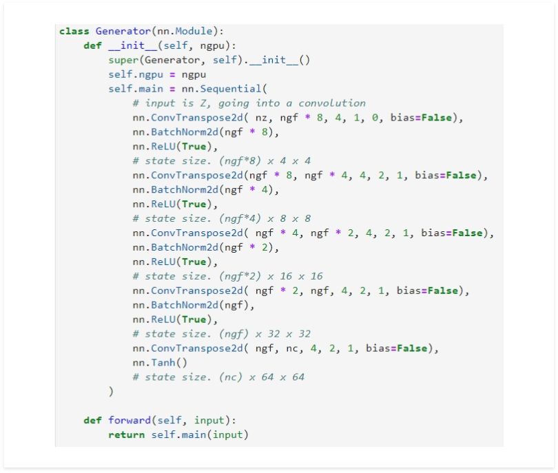
Let’s look at the first layer in the generator. The generator has an input of a 1x1x100 vector (1xnz), and the wanted output is a 3x64x64. We are increasing the dimensionality, so we want to use transposed convolution.

The first convolution uses a kernel size of four, a stride of one and a padding of zero. Let’s plug it in the transposed convolution equation:

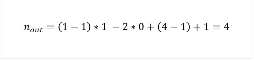
The output size of the transposed convolution is 4x4, as indicated in the code. The next four convolutional layers are identical with a kernel size of four, a stride of two and a padding of one. This doubles the size of each input. So 4x4 turns to 8x8, then 16x16, 32x32 and finally, 64x64.

Without understanding how fully connected layers and convolutional layers are computed and how to calculate the output sizes of convolutional and transposed convolutional layers, one cannot design their own CNN.