

Modern machine translation, search engines, mobile applications, and computer assistants are all equipped with deep learning technology. There are many classic machine learning algorithms and statistical algorithms which can be applied to data. By mimicking the human brain, deep learning models can work wonders when it comes to finding and creating patterns from data.
As deep learning reaches into a plethora of industries, it’s becoming essential for software engineers to develop a work knowledge of its principles. We’ll take an in-depth look at feedforward neural networks, an important part of the core neural network architecture.
Table of Contents
- A quick intro to neural networks
- How feedfoward neural networks work
- Coding a feedforward neural network in TensorFlow
- Summary
A Quick Intro to Neural Networks
Many problems in our daily lives that involve intelligence, pattern recognition, and object detection are challenging to automate, yet seem to be performed quickly and naturally by animals and young children. For example, how does a dog recognize its owner from a complete stranger? How does a child learn to understand the difference between an apple and an orange? The answers lie in the biological neural networks present in our nervous system. These networks do the computations for us and look like this:

An “artificial neural network” is a computation system that attempts to mimic (or at the very least is inspired by) the neural connections in our nervous system. Initially, we used neural networks for simple classification problems, but thanks to an increase in computation power, there are now more powerful architectures that can solve more complex problems. One of these is called a feedforward neural network.
How Feedforward Neural Networks Work
Feedforward neural networks were among the first and most successful learning algorithms. They are also called deep networks, multi-layer perceptron (MLP), or simply neural networks. As data travels through the network’s artificial mesh, each layer processes an aspect of the data, filters outliers, spots familiar entities and produces the final output.
Feedforward neural networks are made up of the following:
- Input layer: This layer consists of the neurons that receive inputs and pass them on to the other layers. The number of neurons in the input layer should be equal to the attributes or features in the dataset.
- Output layer: The output layer is the predicted feature and depends on the type of model you’re building.
- Hidden layer: In between the input and output layer, there are hidden layers based on the type of model. Hidden layers contain a vast number of neurons which apply transformations to the inputs before passing them. As the network is trained, the weights are updated to be more predictive.
- Neuron weights: Weights refer to the strength or amplitude of a connection between two neurons. If you are familiar with linear regression, you can compare weights on inputs like coefficients. Weights are often initialized to small random values, such as values in the range 0 to 1.
To better understand how feedforward neural networks function, let’s solve a simple problem — predicting if it’s raining or not when given three inputs.
- x1 - day/night
- x2 - temperature
- x3 - month
Let’s assume the threshold value to be 20, and if the output is higher than 20 then it will be raining, otherwise it’s a sunny day. Given a data tuple with inputs (x1, x2, x3) as (0, 12, 11), initial weights of the feedforward network (w1, w2, w3) as (0.1, 1, 1) and biases as (1, 0, 0).
Here’s how the neural network computes the data in three simple steps:
1. Multiplication of weights and inputs: The input is multiplied by the assigned weight values, which this case would be the following:
(x1* w1) = (0 * 0.1) = 0
(x2* w2) = (1 * 12) = 12
(x3* w3) = (11 * 1) = 11
2. Adding the biases: In the next step, the product found in the previous step is added to their respective biases. The modified inputs are then summed up to a single value.
(x1* w1) + b1 = 0 + 1
(x2* w2) + b2 = 12 + 0
(x3* w3) + b3 = 11 + 0
weighted_sum = (x1* w1) + b1 + (x2* w2) + b2 + (x3* w3) + b3 = 23
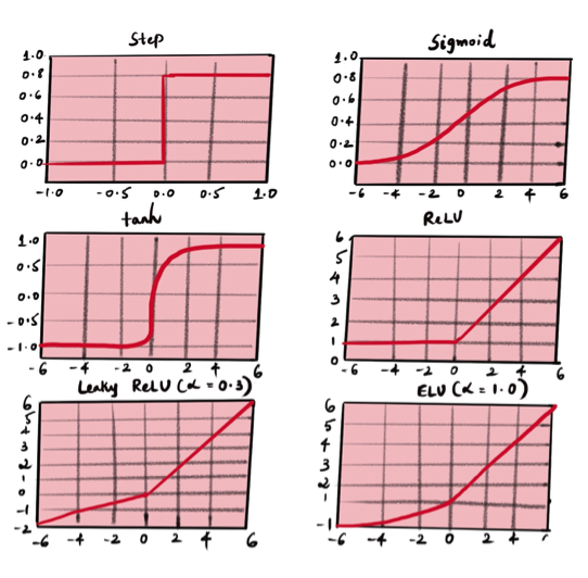
3. Activation: An activation function is the mapping of summed weighted input to the output of the neuron. It is called an activation/transfer function because it governs the inception at which the neuron is activated and the strength of the output signal.
4. Output signal: Finally, the weighted sum obtained is turned into an output signal by feeding the weighted sum into an activation function (also called transfer function). Since the weighted sum in our example is greater than 20, the perceptron predicts it to be a rainy day.
The image below illustrates this process more clearly.

There are several activation functions for different use cases. The most commonly used activation functions are relu, tanh and softmax. Here’s a handy cheat sheet:
Calculating the Loss
In simple terms, a loss function quantifies how “good” or “bad” a given model is in classifying the input data. In most learning networks, the loss is calculated as the difference between the actual output and the predicted output.
Mathematically:
loss = y_{predicted} - y_{original}
The function that is used to compute this error is known as loss function J(.). Different loss functions will return different errors for the same prediction, having a considerable effect on the performance of the model.
Gradient Descent
Gradient descent is the most popular optimization technique for feedforward neural networks. The term “gradient” refers to the quantity change of output obtained from a neural network when the inputs change a little. Technically, it measures the updated weights concerning the change in error. The gradient can also be defined as the slope of a function. The higher the angle, the steeper the slope and the faster a model can learn.
Backpropagation
The predicted value of the network is compared to the expected output, and an error is calculated using a function. This error is then propagated back within the whole network, one layer at a time, and the weights are updated according to the value that they contributed to the error. This clever bit of math is called a backpropagation algorithm. The process is repeated for all of the examples in the training data. One round of updating the network for the entire training dataset is called an epoch. A network may be trained for tens, hundreds or many thousands of epochs.
Coding a Feedforward Neural Network in TensorFlow
In this tutorial, we’ll be using TensorFlow to build our feedforward neural network. Initially, we declare the variable and assign it to the type of architecture we’ll be declaring, which is a “Sequential()” architecture in this case. Next, we directly add layers in a sequential manner using the model.add() method. The type of layer can be imported from tf.layers as shown in the code snippet below. We use adam function as an optimizer and crossentropy function as parameters for our architecture. Once the model is defined, the next step is to start the training process for which we will be using the model.fit() method. The evaluation will be done on the test dataset which can be called using model.evaluate() method.

Using FeedForward Neural Networks
Deep learning is an area of computer science with a huge scope of research. Case in point, there are several neural network architectures implemented for different data types. Convolutional neural networks, for example, have achieved state-of-the-art performance in the fields of image processing techniques, while recurrent neural networks are widely used in text/voice processing.
When applied to large datasets, neural networks need massive amounts of computational power and hardware acceleration, which can be achieved through the configuration of configuring graphics processing units. If you are new to using GPUs you can find free configured settings online. Some of the most used are Kaggle Notebooks/Google Collab Notebooks. To achieve an efficient model one must iterate over network architecture, which needs a lot of experimenting.


