A Guide to Loss Functions for Deep Learning Classification in Python

Deep learning models are a mathematical representation of the network of neurons in the human brain. These models have a wide range of applications in healthcare, robotics, streaming services and much more. For example, deep learning can solve problems in healthcare like predicting patient readmission. Further, Tesla’s self-driving cars employ deep learning models for image recognition. Finally, streaming services like Netflix use these models to analyze subscriber data to suggest new, relevant content to viewers. In all of these situations, the deep learning models fall under a category of machine learning models called classification. 

Machine learning classification is the process of assigning discrete labels to groups in data based on the characteristics of that group. For streaming service platforms, this could mean grouping viewers into buckets like “enjoys comedy series” or  “enjoys romance films.” An important part of this process is to minimize the number of times items are misclassified and placed in the wrong group. In the Netflix example, such misclassification could make the system incorrectly suggest horror content to comedy film lovers. So, for a machine learning model to do a good job at minimizing misclassifications, data scientists need to select the right loss function for the problem they are trying to solve. 

”Loss function” is a fancy mathematical term for an object that measures how often a model makes an incorrect prediction. In the context of classification, they measure how often a model misclassifies members of different groups. The most popular loss functions for deep learning classification models are binary cross-entropy and sparse categorical cross-entropy. 

Binary cross-entropy is useful for binary and multilabel classification problems. For example, predicting whether a moving object is a person or a car is a binary classification problem because there are two possible outcomes. Adding a choice and predicting if an object is a person, car, or building transforms this into a multilabel classification problem. 

Sparse categorical cross-entropy is useful for multiclass classification problems. This is typically framed as a one-versus-the-rest problem where a binary classifier is trained for each class. For example, this model should be able to predict the presence of a car in an image as well as predict if images of a person, buildings, and parks are not cars. Additional binary classifiers are also built for detecting people, buildings and parks. For the first classifier, the prediction labels here correspond to “cars” and “not cars.” For the second classifier, the labels are “person” and “not a person,” and so forth. We can use this method to predict distinct labels (e.g., person, car, building, park) where we’d use the model prediction with the highest probability. It can also be used if we are only interested in distinguishing a single class from all other classes and we don’t care to distinguish the other classes from each other. The latter is how we will be applying this type of model. 

This differs from multilabel classification, which can both predict if an image is of a car and then further distinguish images that are not cars. Given that choosing the right loss function depends on the problem at hand, having a basic understanding of these functions and knowing when to use them is essential for any data scientist. 

The Keras library in Python is an easy-to-use API for building scalable deep learning models. Defining the loss functions in the models is straightforward, as it involves defining a single parameter value in one of the model function calls. 

Here, we will look at how to apply different loss functions for binary and multiclass classification problems. 

For our binary classification model, we will predict customer churn, which happens when a customer cancels a subscription or no longer makes purchases with a company. We will work with the fictional Telco Churn data set. The data set is under the Creative Commons license for data sharing. 

For our multiclass classification problem, we will build a model that predicts handwritten digits. We will be using the publicly available MNIST dataset, which is available in the Keras library, for our multiclass prediction model. 

More From Sadrach PierreAn Introduction to Dimensionality Reduction in Python

Reading in Telco Churn Data 

To start, let's import the Pandas library, which we will use to read our data. Let’s also display the first five rows of data using the Pandas head():

import pandas as pd 

df = pd.read_csv(“telco.csv”)

print(df.head())

We will build a deep learning model that predicts whether a customer will churn. To do this, we need to convert the values of the churn column into machine-readable labels. Wherever the value in the churn column is “no,” we will assign an integer label of “0” and churn values of “yes” will have an integer label of “1.” 

Let’s import the numpy package and use the where() method to label our data:

import numpy as np 
df['Churn'] = np.where(df['Churn'] == 'Yes', 1, 0)

In our deep learning model, we will want to use both categorical and numerical features. Similar to the labels, we need to convert the categorical values into machine-readable numbers that we can use to train our model. Let’s define a simple function that performs this task:

def convert_categories(cat_list):
    for col in cat_list:
        df[col] = df[col].astype('category')
        df[f'{col}_cat'] = df[f'{col}_cat'].cat.codes

Next, we will specify our list of categorical columns, call our function with this list, and display our data frame:

category_list = ['gender', 'Partner', 'Dependents', 'PhoneService', 
'MultipleLines', 'InternetService',
                  'OnlineSecurity', 'OnlineBackup', 
'DeviceProtection', 'TechSupport', 'StreamingTV',
                  'StreamingMovies', 'Contract', 'PaperlessBilling', 
'PaymentMethod']

convert_categories(category_list)

print(df.head())

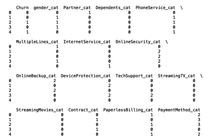
We can see that our data frame now contains categorical codes for each categorical column. 

The next thing we need to do is force the TotalCharges column to be a float since there are some non-numeric, meaning bad, values in this column. Non-numeric values are converted to a “not a number” value (NaN), and we replace the NaN values with 0:

df['TotalCharges'] = pd.to_numeric(df['TotalCharges'], 
errors='coerce')
df['TotalCharges'].fillna(0, inplace=True)

Next, let’s define our input and output:

X = df[['gender_cat', 'Partner_cat', 'Dependents_cat', 
'PhoneService_cat', 'MultipleLines_cat', 'InternetService_cat',
                  'OnlineSecurity_cat', 'OnlineBackup_cat', 
'DeviceProtection_cat', 'TechSupport_cat', 'StreamingTV_cat',
                  'StreamingMovies_cat', 'Contract_cat', 
'PaperlessBilling_cat', 'PaymentMethod_cat','MonthlyCharges'
                  'TotalCharges', 'SeniorCitizen', 'tenure']]

y= df['Churn']

Next, let’s import the train/test split method for the model selection module in Scikit-learn. Let’s also split our data for training and testing

from sklearn.model_selection import train_test_split

X_train, X_test_hold_out, y_train, y_test_hold_out = 
train_test_split(X, y, test_size=0.33)

Deep Neural Network Loss Functions for Classification 

Binary Cross-Entropy 

To start building our network classification model, we will start by importing the dense layer class from the layers module in Keras:

from tensorflow.keras.layers import Dense

Let’s also import the sequential class and the accuracy method from the metrics module:

from tensorflow.keras.models import Sequential
from sklearn.metrics import accuracy_score

Now, let’s build a neural network with three hidden layers and 32 neurons. We will also use 20 epochs, which corresponds to the number of passes through the training data:

We will start by defining a variable called model_bce, which is an instance of the sequential class:

model_bce = Sequential()

Next, we will use the add() method on the sequential class instance to add a dense layer. This will be the input layer to our neural network in which we specify the number of inputs, how we initialize weights, and the activation function:

model_bce.add(Dense(len(cols),input_shape=(len(cols),), 
kernel_initializer='normal', activation='relu')) 

Next, we will add three hidden layers using the add method. These layers will have 32 neurons and also use a ReLu activation function:

model_bce.add(Dense(32, activation='relu'))
model_bce.add(Dense(32, activation='relu'))
model_bce.add(Dense(32, activation='relu'))

We then need to add the output layer, which will have one neuron and a softmax activation function. This will allow our model to output class probabilities for predicting whether a customer will churn:

model_bce.add(Dense(1, activation='softmax'))

Finally, we will use the compile method on our model instance to specify the loss function we will use. To start, we will specify the binary cross-entropy loss function, which is best suited for the type of machine learning problem we’re working on here. 

We specify the binary cross-entropy loss function using the loss parameter in the compile layer. We simply set the “loss” parameter equal to the string “binary_crossentropy”:

model_bce.compile(optimizer = 'adam',loss='binary_crossentropy', 
metrics =['accuracy'])

Finally, we can fit our model to the training data:

model_bce.fit(X_train, y_train,epochs =20)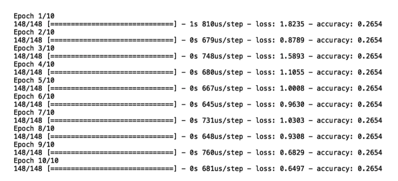

We see that, for each of the 10 epochs, we have a value for our loss function. We also see that, with each epoch, our loss decreases, which means that our model improves over the course of training. 

Binary cross-entropy is most useful for binary classification problems. In our churn example, we were predicting one of two outcomes: either a customer will churn or not. If you’re working on a classification problem where there are more than two prediction outcomes, however, sparse categorical cross-entropy is a more suitable loss function. 

Sparse Categorical Cross-Entropy 

In order to apply the categorical cross-entropy loss function to a suitable use case, we need to use a data set that contains more than two labels. Here, we will work with the MNIST data set, which contains images of hand-written digits between zero and 9. Let’s start by importing the data:

from tensorflow.keras.datasets import mnist

Next, let’s store the input and output:

(X_train_mnist, y_train_mnist), (X_test_mnist, y_test_mnist) = 
mnist.load_data()

We can easily visualize some of the digits in the data using matplotlib:

This image contains a five:

plt.imshow(X_train_mnist[0])
plt.show()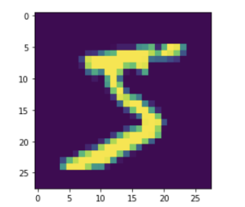

This image contains a zero:

plt.imshow(X_train_mnist[1])
plt.show()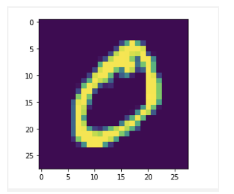

This image contains a nine: 

plt.imshow(X_train_mnist[4])
plt.show()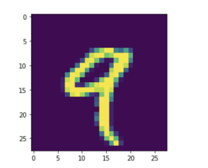

Let’s reformat the data so that we can use it to train our model:

X_train_mnist = X_train_mnist.reshape((X_train_mnist.shape[0], 28, 28, 
1))
X_test_mnist = X_test_mnist.reshape((X_test_mnist.shape[0], 28, 28, 
1))

Next, we need to generate binary labels from our classes. Let’s build a model that predicts whether or not an image contains the number nine. We will assign a label of “1” to images with a number nine. Any other number that is not nine will have a label of “0.” This type of problem is different from multilabel classification where we would have nine labels corresponding to each of the nine digits. 

Let’s generate our binary labels:

y_train_mnist = np.where(y_train_mnist == 9, 1, 0)
y_test_mnist = np.where(y_test_mnist == 9, 1, 0)

Next, we will build a convolutional neural network, which is the typical architecture for image classification. First, let’s import the layers:

from tensorflow.keras.layers import Conv2D, MaxPooling2D, Flatten

Next, let’s initialize the model and add our layers:

model_cce = Sequential()
model_cce.add(Conv2D(16, (3, 3), activation='relu', 
kernel_initializer='normal', input_shape=(28, 28, 1)))
model_cce.add(MaxPooling2D((2, 2)))
model_cce.add(Flatten())
model_cce.add(Dense(16, activation='relu', 
kernel_initializer='normal'))
model_cce.add(Dense(2, activation='softmax'))

In our compile layer, we will specify the sparse categorical cross-entropy loss function:

model_cce.compile(optimizer = 
'SGD',loss='sparse_categorical_crossentropy', metrics =['accuracy'])

And fit our model:

model_cce.fit(X_train_mnist, y_train_mnist, epochs =10)

The code in this post is available on GitHub. 

In our image classification example, we were predicting the labels “contains a nine” and “doesn’t contain a nine.” The “doesn’t contain a nine” label is made up of nine distinct classes. This is in contrast to the negative example in the churn prediction model, where the “doesn’t churn” label corresponds exactly to a single class. In the case of churn, the prediction outcomes were binary. A customer either churns or doesn't, where the “doesn’t churn” label is only made up of a single class. 

More in Data ScienceSQL vs. NoSQL: Which Should You Choose?

Experiment With Loss Functions

Knowing which loss function to use for different types of classification problems is an important skill for every data scientist. Understanding the difference between types of classification informs the choice of loss function for a neural network model and how machine learning problems are framed. How a data science team frames a machine learning problem can have a significant impact on the value added to the company. Consider the churn example, with three classes for the probability of churn: low, medium and high. One company may be interested in developing ad campaigns that target each distinct group, which requires a multilabel classification model. 

Another company may only be interested in targeting customers with a high probability of churn, not caring to distinguish low from medium. This would require a multiclass classification model. These two types of classification problems add value in different ways and which is most appropriate depends on the business use case. For that reason, knowing the difference between these types of prediction problems and which loss function is appropriate for each is important.