The transformer neural network is a novel architecture that aims to solve sequence-to-sequence tasks while handling long-range dependencies with ease. It was first proposed in the paper “Attention Is All You Need” and is now a state-of-the-art technique in the field of natural language processing (NLP).
Before jumping into the transformer network, I will explain why we use it and where it comes from. So, the story starts with recurrent neural networks (RNNs).
What is the transformer neural network?
Recurrent Neural Network
What is a recurrent neural network (RNN)? How is it different from a simple artificial neural network (ANN)? What is the major difference?
RNNs are feed-forward neural networks that are rolled out over time.
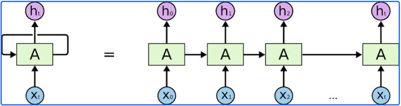
Unlike normal neural networks, RNNs are designed to take a series of inputs with no predetermined limit on size. The term “series” here denotes that each input of that sequence has some relationship with its neighbors or has some influence on them.

Basic feed-forward networks “remember” things too, but they remember the things they learned during training. Although RNNs learn similarly during training, they also remember things learned from prior input(s) while generating output(s).
RNNs can be used in multiple types of models.
1. Vector-Sequence Models — Take fixed-sized vectors as input and output vectors of any size. For example, in image captioning, the image is the input and the output describes the image.
2. Sequence-Vector Model — Take a vector of any size and output a vector of fixed size. For example, sentiment analysis of a movie rates the review of any movie, positive or negative, as a fixed size vector.
3. Sequence-to-Sequence Model — The most popular and most used variant, this takes a sequence as input and outputs another sequence with variant sizes. An example of this is language translation for time series data for stock market prediction.
An RNN has two major disadvantages, however:
- It’s slow to train.
- Long sequences lead to vanishing gradient or the problem of long-term dependencies. In simple terms, its memory is not that strong when it comes to remembering old connections.
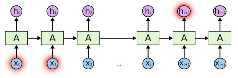
For example, in the sentence “The clouds are in the ____,” the next word should obviously be sky, as it is linked with the clouds. If the distance between clouds and the predicted word is short, the RNN can predict it easily.
Consider another example, however: “I grew up in Germany with my parents, I spent many years there and have proper knowledge about their culture. That’s why I speak fluent ____.”
Here the predicted word is German, which is directly connected with Germany. The distance between Germany and the predicted word is longer in this case, however, so it’s difficult for the RNN to predict.
So, unfortunately, as that gap grows, RNNs become unable to connect as their memory fades with distance.
Long Short-Term Memory

Long short-term memory (LSTM) is a special kind of RNN, specially made for solving vanishing gradient problems. They are capable of learning long-term dependencies. In fact, remembering information for long periods of time is practically their default behavior, not something they struggle to learn!

LSTM neurons, unlike the normal version, have a branch that allows passing information to skip the long processing of the current cell. This branch allows the network to retain memory for a longer period of time. It improves the vanishing gradient problem but not terribly well: It will do fine until 100 words, but around 1,000 words, it starts to lose its grip.
Further, like the simple RNN, it is also very slow to train, and perhaps even slower. These systems take input sequentially one by one, which doesn’t use up GPUs very well, which are designed for parallel computation. Later, I’ll address how we can parallelize sequential data. For now, we are dealing with two issues:
- Vanishing gradient
- Slow training
Solving the Vanishing Gradient Issue
Attention answers the question of what part of the input we should focus on. I’m going to explain attention via a hypothetical scenario:
Suppose someone gave us a book on machine learning and asked us to compile all the information about categorical cross-entropy. There are two ways of doing such a task. First, we could read the whole book and come back with the answer. Second, we could skip to the index, find the chapter on losses, go to the cross-entropy part and just read the relevant information on categorical cross-entropy.
Which do you think is the faster method?
The first approach may take a whole week, whereas the second should just take a few minutes. Furthermore, our results from the first method will be vaguer and full of too much information. The second approach will more accurately meet the requirement.
What did we do differently here?
In the former case, we didn’t zero in on any one part of the book. In the latter method, however, we focused our attention on the losses chapter and more specifically on the part where the concept of categorical cross-entropy is explained. This second version is the way most of us humans would actually do this task.
Attention in neural networks is somewhat similar to what we find in humans. It means they focus on certain parts of the inputs while the rest gets less emphasis.
Let’s say we are making an NMT (neural machine translator). This animation shows how a simple seq-to-seq model works.
We see that, for each step of the encoder or decoder, the RNN is processing its inputs and generating output for that time step. In each time step, the RNN updates its hidden state based on the inputs and previous outputs it has seen. In the animation, we see that the hidden state is actually the context vector we pass along to the decoder.
Time for Attention
The context vector turns out to be problematic for these types of models, which struggle when dealing with long sentences. Or they may have been facing the vanishing gradient problem in long sentences. So, a solution came along in a paper that introduced attention. It highly improved the quality of machine translation as it allows the model to focus on the relevant part of the input sequence as necessary.
This attention model is different from the classic seq-to-seq model in two ways. First, as compared to a simple seq-to-seq model, here, the encoder passes a lot more data to the decoder. Previously, only the final, hidden state of the encoding part was sent to the decoder, but now the encoder passes all the hidden states, even the intermediate ones.
The decoder part also does an extra step before producing its output. This step proceeds like this:
- It checks each hidden state that it received as every hidden state of the encoder is mostly associated with a particular word of the input sentence.
- It give each hidden state a score.
- Each score is multiplied by its respective softmax score, thus amplifying hidden states with high scores and drowning out hidden states with low scores. A clear visualization is available here.
This scoring exercise happens at each time step on the decoder side.
Now, when we bring the whole thing together:
- The attention decoder layer takes the embedding of the <END> token and an initial decoder hidden state. The RNN processes its inputs and produces an output and a new hidden state vector (h4).
- Now, we use encoder hidden states and the h4 vector to calculate a context vector, C4, for this time step. This is where the attention concept is applied, giving it the name the attention step.
- We concatenate (h4) and C4 in one vector.
- Now, this vector is passed into a feed-forward neural network. The output of the feed-forward neural networks indicates the output word of this time step.
- These steps get repeated for the next time steps. A clear visualization is available here.
So, this is how attention works. For further clarification, you can see its application to an image captioning problem here.
Now, remember earlier I mentioned parallelizing sequential data? Here comes our ammunition for doing just that.
Transformers
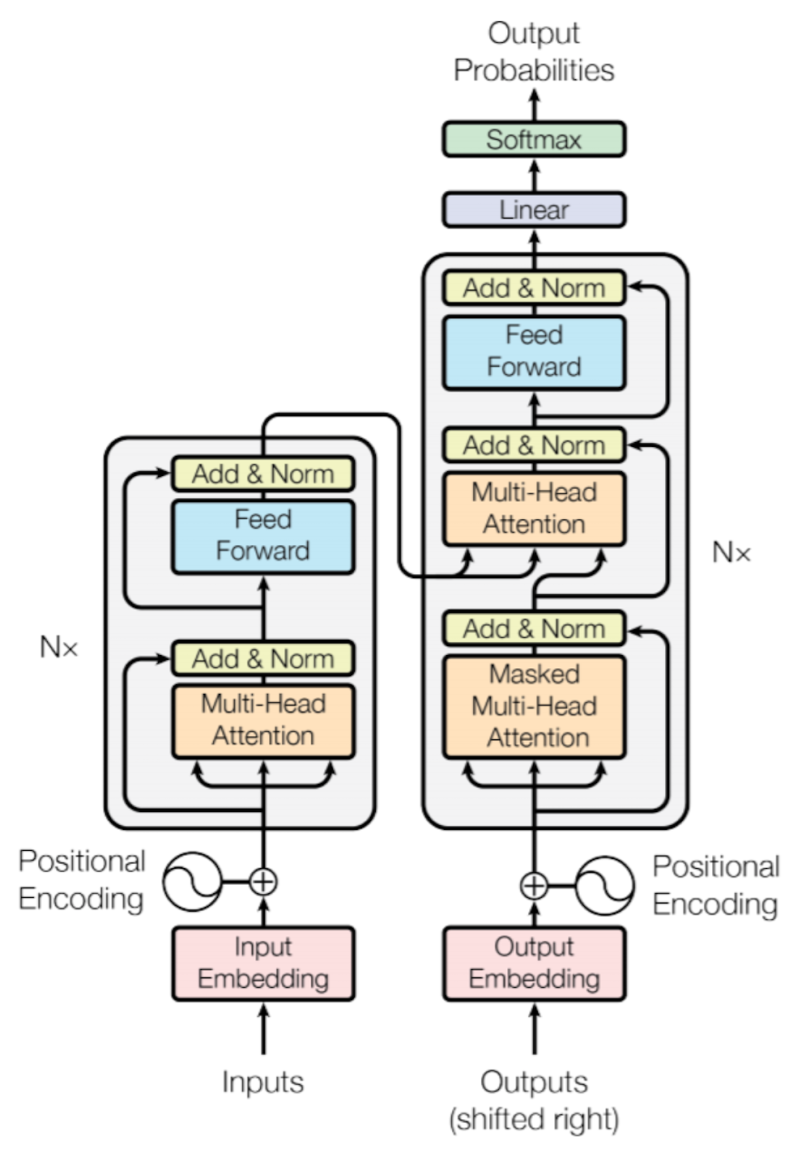
A paper called “Attention Is All You Need,” published in 2017, introduced an encoder-decoder architecture based on attention layers, which the authors called the transformer.
One main difference is that the input sequence can be passed parallelly so that GPU can be used effectively and the speed of training can also be increased. It is also based on the multi-headed attention layer, so it easily overcomes the vanishing gradient issue. The paper applies the transformer to an NMT.
So, both of the problems that we highlighted before are partially solved here.
For example, in a translator made up of a simple RNN, we input our sequence or the sentence in a continuous manner, one word at a time, to generate word embeddings. As every word depends on the previous word, its hidden state acts accordingly, so we have to feed it in one step at a time.
In a transformer, however, we can pass all the words of a sentence and determine the word embedding simultaneously. So, let’s see how it’s actually working:
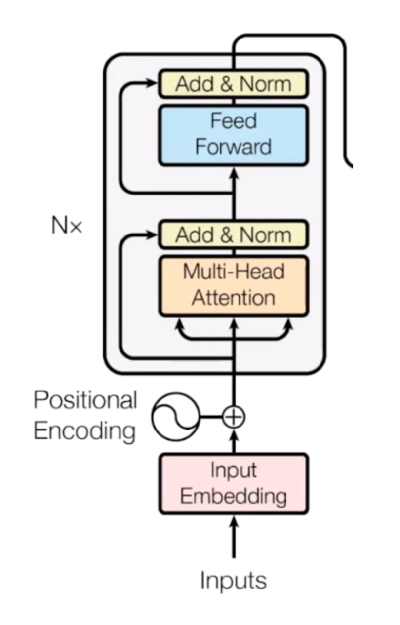
Encoder Block
Computers don’t understand words. Instead, they work on numbers, vectors or matrices. So, we need to convert our words to a vector. But how is this possible? Here’s where the concept of embedding space comes into play. It’s like an open space or dictionary where words of similar meanings are grouped together. This is called an embedding space, and here every word, according to its meaning, is mapped and assigned with a particular value. Thus, we convert our words into vectors.

One other issue we will face is that, in different sentences, each word may take on different meanings. So, to solve this issue, we use positional encoders. These are vectors that give context according to the position of the word in a sentence.
Word → Embedding → Positional Embedding → Final Vector, framed as Context.
So, now that our input is ready, it goes to the encoder block.
Multi-Head Attention Part

Now comes the main essence of the transformer: self attention.
This focuses on how relevant a particular word is with respect to other words in the sentence. It is represented as an attention vector. For every word, we can generate an attention vector generated that captures the contextual relationship between words in that sentence.
The only problem now is that, for every word, it weighs its value much higher on itself in the sentence, but we want to know its interaction with other words of that sentence. So, we determine multiple attention vectors per word and take a weighted average to compute the final attention vector of every word.
As we are using multiple attention vectors, this process is called the multi-head attention block.
Feed-Forward Network
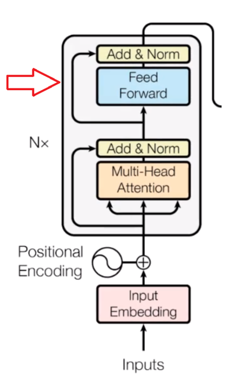
Now, the second step is the feed-forward neural network. A simple feed-forward neural network is applied to every attention vector to transform the attention vectors into a form that is acceptable to the next encoder or decoder layer.

The feed-forward network accepts attention vectors one at a time. And the best thing here is, unlike the case of the RNN, each of these attention vectors is independent of one another. So, we can apply parallelization here, and that makes all the difference.

Now we can pass all the words at the same time into the encoder block and get the set of encoded vectors for every word simultaneously.
Decoder Block

Now, if we’re training a translator for English to French, for training, we need to give an English sentence along with its translated French version for the model to learn. So, our English sentences pass through encoder block, and French sentences pass through the decoder block.

At first, we have the embedding layer and positional encoder part, which changes the words into respective vectors. This is similar to what we saw in the encoder part.
Masked Multi-Head Attention Part

Now it will pass through the self-attention block, where attention vectors are generated for every word in the French sentences to represent how much each word is related to every word in the same sentence, just like we saw in the encoder part.
But this block is called the masked multi-head attention block, which I am going to explain in simple terms. First, we need to know how the learning mechanism works. When we provide an English word, it will be translated into its French version using previous results. It will then match and compare with the actual French translation that we fed into the decoder block. After comparing both, it will update its matrix value. This is how it will learn after several iterations.
What we observe is that we need to hide the next French word so that, at first, it will predict the next word itself using previous results without knowing the real translated word. For learning to take place, it would make no sense if it already knows the next French word. Therefore, we need to hide (or mask) it.
We can take any word from the English sentence, but we can only take the previous word of the French sentence for learning purposes. So, while performing parallelization with the matrix operation, we need to make sure that the matrix will mask the words appearing later by transforming them into zeroes so that the attention network can’t use them.

Now, the resulting attention vectors from the previous layer and the vectors from the encoder block are passed into another multi-head attention block. This is where the results from the encoder block also come into the picture. In the diagram, the results from the encoder block also clearly come here. That’s why it is called the encoder-decoder attention block.
Since we have one vector of every word for each English and French sentence, this block actually does the mapping of English and French words and finds out the relation between them. So, this is the part where the main English to French word mapping happens.
The output of this block is attention vectors for every word in the English and French sentences. Each vector represents the relationship with other words in both languages.
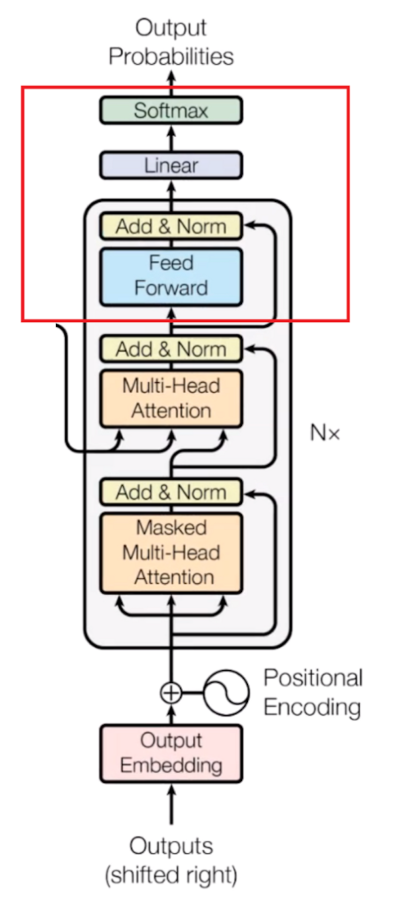
Now, if we pass each attention vector into a feed-forward unit, it will make the output vectors into a form that is easily acceptable by another decoder block or a linear layer. A linear layer is another feed-forward layer that expands the dimensions into numbers of words in the French language after translation.
Now it is passed through a softmax layer that transforms the input into a probability distribution, which is human interpretable, and the resulting word is produced with the highest probability after translation.
Here is an example from Google’s AI blog. In the animation, the transformer starts by generating initial representations, or embeddings, for each word that are represented by the unfilled circles. Then, using self-attention, it aggregates information from all of the other words, generating a new representation per word informed by the entire context, represented by the filled balls. This step is then repeated multiple times in parallel for all words, successively generating new representations.
The decoder operates similarly, but generates one word at a time, from left to right. It attends not only to the other previously generated words but also to the final representations generated by the encoder.
The Takeaway
So, this is how the transformer works, and it is now the state-of-the-art technique in NLP. Its results, using a self-attention mechanism, are promising, and it also solves the parallelization issue. Even Google uses BERT, which uses a transformer to pre-train models for common NLP applications.
Frequently Asked Questions
What is a transformer in neural networks?
A transformer is a type of neural network architecture that transforms an input sequence into an output sequence. It performs this by tracking relationships within sequential data, like words in a sentence, and forming context based on this information. Transformers are often used in natural language processing to translate text and speech or answer questions given by users.
Is transformer better than CNN?
Both vision transformers and CNNs (convolutional neural networks) can be used for image classification and object detection tasks. Vision transformers may excel in contextual understanding and capturing global dependencies in datasets. CNNs may be less memory-intensive, require less training data and handle large datasets effectively in comparison to transformers.
What is the difference between RNN and transformer?
An RNN (recurrent neural network) processes sequences step-by-step or sequentially. A transformer uses self-attention mechanisms to process sequences in parallel, meaning multiple different parts of a sequence are processed at the same time.
What is the difference between LSTM and transformer?
LSTM (long short-term memory) is a type of recurrent neural network effective for capturing long-term dependencies in sequences, with less of a vanishing gradient problem than that of traditional RNNs. Transformers are effective at capturing long-range dependencies without using recurrence, and processes its data in parallel.