Complete Guide to the Adam Optimization Algorithm

Optimization algorithms are the bread and butter of deep learning. We use them whenever we train any neural network and modify the model parameters to minimize loss. But one algorithm stands out for training neural networks  —  Adam optimization. Adam, which stands for Adaptive Moment Estimation, is particularly well-suited for training deep neural networks because it computes individual adaptive learning rates for different parameters.

This post will try to demystify Adam and see what makes it tick. We will look at how it adapts learning rates, the theory behind it, its configuration parameters, and an example of how we can use it. We will also highlight the advantages of Adam over other optimization methods and where it’s commonly applied. 

So, let’s unravel the inner workings of Adam.

More From Rahul AgarwalA Complete Guide to PySpark Dataframes

What Is the Adam Optimization Algorithm?

Adam is an adaptive learning rate algorithm designed to improve training speeds in deep neural networks and reach convergence quickly. It was introduced in the paper “Adam: A Method for Stochastic Optimization.” 

But before we jump into Adam, let’s start with standard gradient descent. It lays the foundation for Adam, which is essentially an adaptive extension of the same algorithm. Standard gradient descent is represented by the following equation:

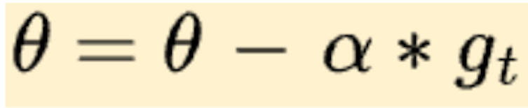
Here, θ = Model parameters, α = Learning rate, and gₜ = Gradient of the cost function with respect to the parameters.

This update changes the parameters θ in the negative direction of the gradient to minimize the cost function. The learning rate α determines the size of the step.

In the standard gradient descent algorithm, the learning rate α is fixed, meaning we need to start at a high learning rate and manually change the alpha by steps or by some learning schedule. A lower learning rate at the onset would lead to very slow convergence, while a very high rate at the start might miss the minima. 

Adam solves this problem by adapting the learning rate α for each parameter θ, enabling faster convergence compared to standard gradient descent with a constant global learning rate.

How Does Adam Optimization Work?

So, that is all great, but how does this adaptive learning rate strategy work? Let’s try to understand it through an example. Think of Adam as a father teaching his two kids, Chris and Sam, how to ride bikes. They have a problem, though: While Chris is afraid to pick up speed on his bike, Sam is more daring and pedals very fast. If Adam pushes both bikes at the same speed, Chris will lag because he’s too slow, while Sam might crash going too fast! 

So, Adam keeps noting the speed and acceleration of each kid and uses that information to adapt his strategy to push them. He notices that Chris has been going slow in general. So, he gently pushes Chris’s bike harder to speed him up. Likewise, he sees Sam has been pedaling very quickly, so he lightly pushes Sam’s bike to slow him down a bit. By adaptively adjusting the speed for each kid, he can train both of them at the right pace. Chris picks up speed comfortably while Sam avoids accidents. 

The Adam optimization works similarly. It customizes each parameter’s learning rate based on its gradient history, and this adjustment helps the neural network learn efficiently as a whole.

More in Machine LearningThe Ultimate Guide to MidJourney V5

Theory Behind Adam

So, now that we have a high-level view, we can delve into the gnarly mathematical details of how Adam achieves this feat. But before we do, we still need to understand two important concepts about optimization algorithms that came before Adam and that, in conjunction, make up the Adam optimization algorithm.

1. Momentum

Momentum speeds up training by accelerating gradients in the right directions by adding a fraction of the previous gradient to the current one. For example, let’s say a gradient has been consistently pointing in the same direction. The momentum term proportional to the previous gradients will accumulate and accelerate the optimization in that direction. 

So, assume that the gradient descent algorithm is working to roll a ball down a hill. Normally, it will take fixed steps as the learning rate is the same throughout. That means you calculate the gradient at each step and take a step in that direction of value α. The Momentum technique helps you to realize that, since the last few steps have been pretty much in the same direction, you could apply a boost to the current step to move in that direction so you need to take fewer steps.

Here is the same in mathematical terms:

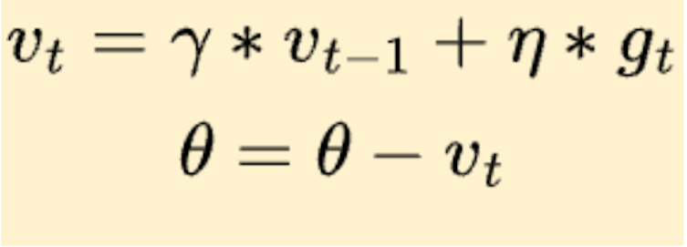
So, what we’re doing here is effectively subtracting the momentum update from θ now compared to the gradient descent algorithm. Also, we can see how the momentum vector v at time t, vₜ is a function of the previous momentum vector vₜ₋₁. The hyperparameter γ is the momentum decay that exponentially decays the past momentum vector, and η is the learning rate used to take the step in the opposite direction of the gradient. 

2. Root Mean Square Propagation (RMSProp):

Using Momentum, we effectively increase our learning rate if the previous gradients are in the same direction. In RMSProp, we look at the “steepness” of the error surface for each parameter to update the learning rate adaptively. Parameters with high gradients get smaller update steps, and low gradients allow bigger steps. So, while Momentum is about accelerating in consistent directions, RMSProp is based on controlling overshooting by modulating step size. Here is the formula for the update:

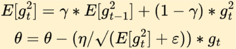
The first equation is a weighted moving average of squared gradients, which effectively is the variance of gradients. Here we see that the learning rate in the θ update is divided by the square root of the moving average of the squared gradients. This means that, when the variance of gradients is high, we reduce the learning rate as we want to be more conservative. And when the variance of gradients is low, we increase the learning rate, thus going faster towards the optima.

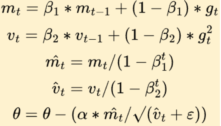
So, now we understand the Momentum and RMSProp, and we can see how Adam works. Here is the simplified version of Adam:

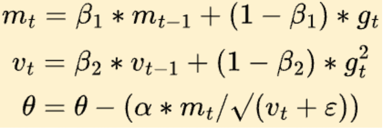
Adam combines the two approaches through hyperparameters β₁ and β₂. We can see how the θ update looks similar to the RMSProp update, amplified with Momentum, so we get the best of both words.

In its final version, Adam also introduces a warm start. The t value varies from one to num_steps. It warm starts the algorithm when the start mₜ₋₁ and vₜ₋₁ values are zero. 

Adam Configuration Parameters

So, now that we understand everything about Adam, we can look at the various hyperparameters in the Adam equation.

The main hyperparameters in Adam are:

• α — Step size for the optimization.
• β₁ — Decay rate for momentum. The typical value is 0.9 as we want to have high weighting for the most recent gradients.
• β₂ — Decay rate for squared gradients. The typical value is 0.999. This is because 0.999 captures the long-term memory of gradients. We want a stable estimate of variance.
• ϵ— Small value to prevent division by zero. It is usually around 1e-8.

Together, these parameters enable Adam to converge faster while remaining numerically stable. The defaults work well for most cases but can be tuned if needed.

Adam Optimization Algorithm Example

Adam is, by default, implemented in most of the frameworks for deep learning. Here is an example of how we can use Adam in PyTorch.

import torch
import torch.nn as nn
from torch.optim import Adam

# Model and loss function
model = nn.Sequential(nn.Linear(10, 5), 
                      nn.ReLU(),
                      nn.Linear(5, 1))
criterion = nn.MSELoss()

# Optimizer
optimizer = Adam(model.parameters(), lr=0.001, betas=(0.9, 0.999)) 

# Training loop
for epoch in range(100):
  # Forward pass
  outputs = model(inputs)
  loss = criterion(outputs, targets)
  
  # Backward pass and optimize
  optimizer.zero_grad()
  loss.backward()
  optimizer.step()

Advantages of Adam Optimization

Some key advantages of Adam optimization include the following:

• Faster convergence — By adapting the learning rate during training, Adam converges much more quickly than SGD.
• Easy to implement — Only requiring first-order gradients, Adam is straightforward to implement and combine with deep neural networks. A few lines of code using Python and PyTorch are all you need.
• Robust algorithm — Adam performs well across various model architectures.
• Little memory requirements — Adam requires storing just the first and second moments of the gradients, keeping memory needs low.
• Wide community adoption — Adam is used extensively by deep learning practitioners and has become a default, go-to optimizer.

Applications of Adam Optimization

Here are some of the key domains and applications where Adam optimization shines for training deep learning models:

• Computer Vision — Adam is ubiquitous in training convolutional neural networks for image classification, object detection, segmentation, and other computer vision tasks.
• Natural Language Processing — For training recurrent neural networks like LSTMs and transformers for language modeling, translation, and text generation.
• Generative Models — Adam is the default optimizer for training generative adversarial networks and variational autoencoders.
• Reinforcement Learning — Algorithms like deep Q-learning use Adam to train neural networks representing policies and value functions.
• Time Series Forecasting — Adam accelerates training sequence models like RNNs for forecasting tasks.
• Recommendation Systems — Adam is useful in training embedding layers and neural collaborative filtering models for recommendations.
• Robotics — In combination with policy gradient methods, Adam can train policies that can control robots.
• Financial Trading — Adam is used with deep reinforcement learning for automated trading systems.

Adam is ubiquitous in nearly every deep learning domain due to its rapid training convergence for high-dimensional parametric models.

Alternatives to Adam Optimization

Because Adam is an optimization method, you can replace it with other optimization methods with varying degrees of success. Here are some alternative optimization algorithms to Adam in deep learning:

• SGD with Momentum — Stochastic gradient descent with Momentum is a simple approach that Adam improves upon.
• Nesterov Accelerated Gradient (NAG) — NAG modifies SGD by computing gradients after a look-ahead step. 
• AdaGrad — AdaGrad adapts learning rates based on summing the squares of all previous gradients for each parameter. 
• RMSprop— As we already know, RMSprop uses a moving average of squared gradients to normalize the gradients and adapt the learning rate per parameter. A fun fact is that this was first explained in a lecture by Geoffrey Hinton, and now everyone cites  “Neural Network for Machine Learning, lecture six” whenever they cite RMSProp in their paper.
• AdaDelta — AdaDelta further adapts RMSprop learning rates based on a window of previous gradient updates. This method does not require a default learning rate.
• AMSGrad — This approach rectifies Adam’s shortcomings in convex settings by using the maximum of past-second moment estimates, not the exponential average.
• NAdam —This method iIncorporates Nesterov momentum into Adam and works better than vanilla Adam in some cases.

In general, Adam is better than other adaptive learning rate algorithms due to its faster convergence and robustness across problems. As such, it’s mostly the default algorithm used for deep learning. But alternatives like NAdam and AMSGrad can outperform Adam in some cases, so trying these would also make sense.

Learning About Machine LearningSigmoid Activation Function: An Introduction

Use the Adam Optimization

I hope this post demystified how Adam delivers state-of-the-art results. We went under the hood to understand how Adam adapts learning rates using the gradients. The intuitive concepts behind Momentum, RMSprop, and bias correction combine elegantly in Adam to accelerate training.

Adam’s remarkable effectiveness across computer vision, NLP, and other domains has made it the go-to algorithm for training deep neural networks. The days of hand-tuning learning rates for SGD are behind us. Now you can leverage Adam to smoothly traverse the loss landscape and reach new heights in deep learning.