A Complete Guide to PySpark DataFrames

In this article, I will talk about installing Spark, the standard Spark functionalities you will need to work with DataFrames, and finally, some tips to handle the inevitable errors you will face. This article is going to be quite long, so go on and pick up a coffee first.

Here is a breakdown of the topics we’ll cover:

More From Rahul AgarwalHow to Set Environment Variables in Linux

 

1. Installation of Apache Spark

I am installing Spark on Ubuntu 18.04, but the steps should remain the same for Macs too. I’m assuming that you already have Anaconda and Python3 installed. After that, you can just go through these steps:

First, download the Spark Binary from the Apache Spark website. Click on the download Spark link.

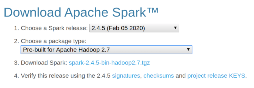
Once you’ve downloaded the file, you can unzip it in your home directory. Just open up the terminal and put these commands in.

cd ~
cp Downloads/spark-2.4.5-bin-hadoop2.7.tgz ~
tar -zxvf spark-2.4.5-bin-hadoop2.7.tgz

Next, check your Java version. As of version 2.4, Spark works with Java 8. You can check your Java version using the command java -version on the terminal window.

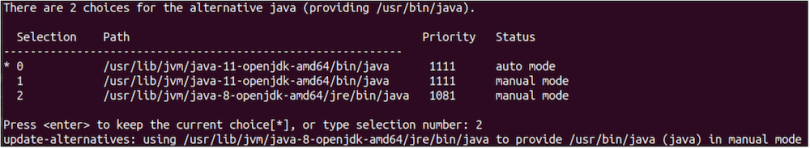
I had Java 11 on my machine, so I had to run the following commands on my terminal to install and change the default to Java 8:

sudo apt install openjdk-8-jdk
sudo update-alternatives --config java

You will need to manually select Java version 8 by typing the selection number.

Rechecking Java version should give something like this:

Next, edit your ~/.bashrc file and add the following lines at the end of it:

function pysparknb () 
{
#Spark path
SPARK_PATH=~/spark-2.4.5-bin-hadoop2.7
export PYSPARK_DRIVER_PYTHON="jupyter"
export PYSPARK_DRIVER_PYTHON_OPTS="notebook"
# For pyarrow 0.15 users, you have to add the line below or you will get an error while using pandas_udf 
export ARROW_PRE_0_15_IPC_FORMAT=1
# Change the local[10] to local[numCores in your machine]
$SPARK_PATH/bin/pyspark --master local[10]
}

Next, run source ~/.bashrc:

source ~/.bashrc

Finally, run the pysparknb function in the terminal, and you’ll be able to access the notebook. You’ll also be able to open a new notebook since the sparkcontext will be loaded automatically.

pysparknb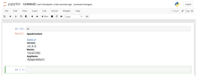

 

2. Data Importation

With the installation out of the way, we can move to the more interesting part of this article. I will be working with the data science for Covid-19 in South Korea data set, which is one of the most detailed data sets on the internet for Covid.

Please note that I will be using this data set to showcase some of the most useful functionalities of Spark, but this should not be in any way considered a data exploration exercise for this amazing data set.

I will mainly work with the following three tables in this piece:

• Cases
• Region
• TimeProvince

You can find all the code at the GitHub repository.

 

3. Basic Functions of Spark

Now, let’s get acquainted with some basic functions.

 

Read

We can start by loading the files in our data set using the spark.read.load command. This command reads parquet files, which is the default file format for Spark, but you can also add the parameter format to read .csv files using it.

cases = 
spark.read.load("/home/rahul/projects/sparkdf/coronavirusdataset/Case.
csv",format="csv", sep=",", inferSchema="true", header="true")

See a few rows in the file:

cases.show()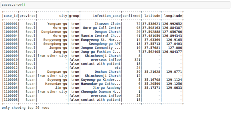

This file contains the cases grouped by way of infection spread. This arrangement might have helped in the rigorous tracking of coronavirus cases in South Korea.

This file looks great right now. Sometimes, though, as we increase the number of columns, the formatting devolves. I’ve noticed that the following trick helps in displaying in Pandas format in my Jupyter Notebook. The .toPandas() function converts a Spark DataFrame into a Pandas version, which is easier to show.

cases.limit(10).toPandas()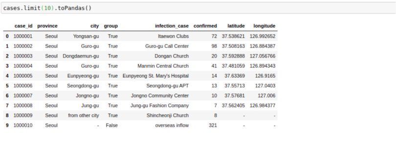

 

Change Column Names

Sometimes, we want to change the name of the columns in our Spark DataFrames. We can do this easily using the following command to change a single column:

cases = cases.withColumnRenamed("infection_case","infection_source")

Or for all columns:

cases = cases.toDF(*['case_id', 'province', 'city', 'group', 
'infection_case', 'confirmed',
       'latitude', 'longitude'])

 

Select Columns

We can also select a subset of columns using the select keyword.

cases = cases.select('province','city','infection_case','confirmed')
cases.show()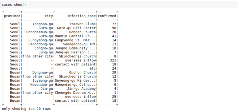

 

Sort

We can sort by the number of confirmed cases. Note here that the cases DataFrame won’t change after performing this command since we don’t assign it to any variable.

cases.sort("confirmed").show()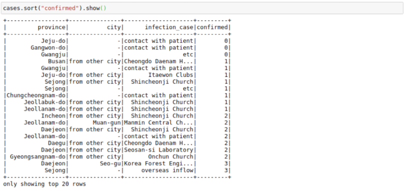

But those results are inverted. We want to see the most cases at the top, which we can do using the F.desc function:

# descending Sort
from pyspark.sql import functions as F
cases.sort(F.desc("confirmed")).show()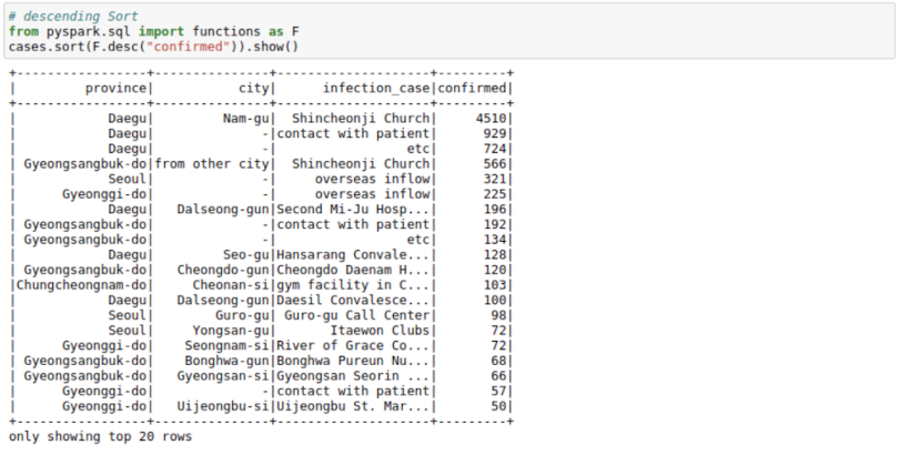

We can see that most cases in a logical area in South Korea originated from Shincheonji Church.

 

Cast

Though we don’t face it in this data set, we might find scenarios in which Pyspark reads a double as an integer or string. In such cases, you can use the cast function to convert types.

from pyspark.sql.types import DoubleType, IntegerType, StringType
cases = cases.withColumn('confirmed', 
F.col('confirmed').cast(IntegerType()))
cases = cases.withColumn('city', F.col('city').cast(StringType()))

 

Filter

We can filter a DataFrame using AND(&), OR(|) and NOT(~) conditions. For example, we may want to find out all the different results for infection_case in Daegu Province with more than 10 confirmed cases.

cases.filter((cases.confirmed>10) & (cases.province=='Daegu')).show()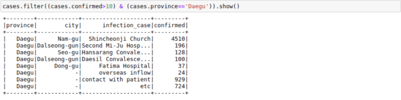

 

GroupBy

We can use groupBy function with a Spark DataFrame too. The process is pretty much same as the Pandas groupBy version with the exception that you will need to import pyspark.sql.functions. Here is a list of functions you can use with this function module.

from pyspark.sql import functions as F
cases.groupBy(["province","city"]).agg(F.sum("confirmed") 
,F.max("confirmed")).show()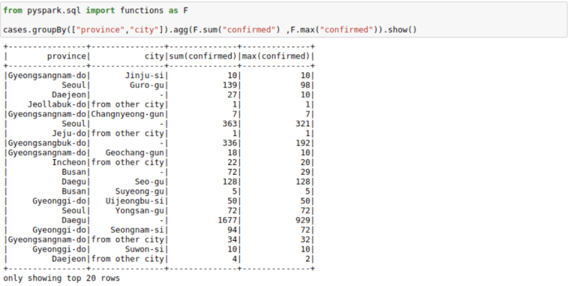

If you don’t like the new column names, you can use the alias keyword to rename columns in the agg command itself.

cases.groupBy(["province","city"]).agg(
    F.sum("confirmed").alias("TotalConfirmed"),\
    F.max("confirmed").alias("MaxFromOneConfirmedCase")\
    ).show()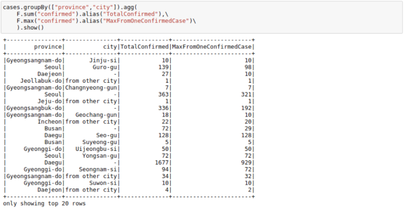

 

Joins

To start with Joins, we’ll need to introduce one more CSV file. We’ll go with the region file, which contains region information such as elementary_school_count, elderly_population_ratio, etc.

regions = 
spark.read.load("/home/rahul/projects/sparkdf/coronavirusdataset/Regio
n.csv",format="csv", sep=",", inferSchema="true", header="true")
regions.limit(10).toPandas()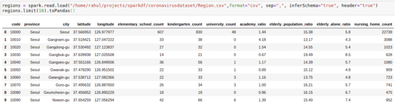

We want to get this information in our cases file by joining the two DataFrames. We can do this by using the following process:

cases = cases.join(regions, ['province','city'],how='left')
cases.limit(10).toPandas()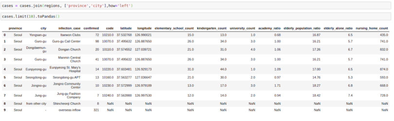

More in Data ScienceTransformer Neural Networks: A Step-by-Step Breakdown

 

4. Broadcast/Map Side Joins in PySpark DataFrames

Sometimes, we might face a scenario in which we need to join a very big table (~1B rows) with a very small table (~100–200 rows). The scenario might also involve increasing the size of your database like in the example below.

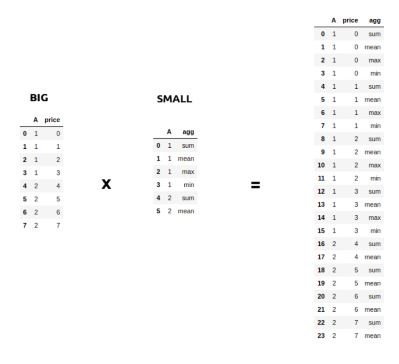
Such operations are aplenty in Spark where we might want to apply multiple operations to a particular key. But assuming that the data for each key in the big table is large, it will involve a lot of data movement, sometimes so much that the application itself breaks. A small optimization that we can do when joining such big tables (assuming the other table is small) is to broadcast the small table to each machine/node when performing a join. We can do this easily using the broadcast keyword. This has been a lifesaver many times with Spark when everything else fails.

from pyspark.sql.functions import broadcast
cases = cases.join(broadcast(regions), ['province','city'],how='left')

 

5. Use SQL With PySpark DataFrames

If we want, we can also use SQL with DataFrames. Let’s try to run some SQL on the cases table.

We first register the cases DataFrame to a temporary table cases_table on which we can run SQL operations. As we can see, the result of the SQL select statement is again a Spark DataFrame.

cases.registerTempTable('cases_table')
newDF = sqlContext.sql('select * from cases_table where 
confirmed>100')
newDF.show()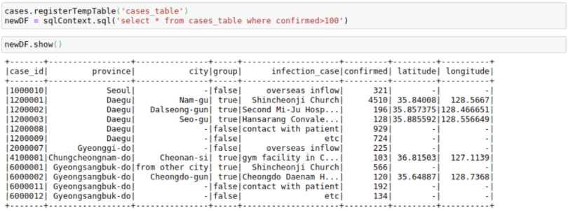

I have shown a minimal example above, but we can use pretty much any complex SQL queries involving groupBy, having and orderBy clauses as well as aliases in the above query.

 

6. Create New Columns in PySpark DataFrames

We can create a column in a PySpark DataFrame in many ways. I will try to show the most usable of them.

 

Using Spark Native Functions

The most PySparkish way to create a new column in a PySpark DataFrame is by using built-in functions. This is the most performant programmatical way to create a new column, so it’s the first place I go whenever I want to do some column manipulation.

We can use .withcolumn along with PySpark SQL functions to create a new column. In essence, we can find String functions, Date functions, and Math functions already implemented using Spark functions. Our first function, F.col, gives us access to the column. So, if we wanted to add 100 to a column, we could use F.col as:

import pyspark.sql.functions as F
casesWithNewConfirmed = cases.withColumn("NewConfirmed", 100 + 
F.col("confirmed"))
casesWithNewConfirmed.show()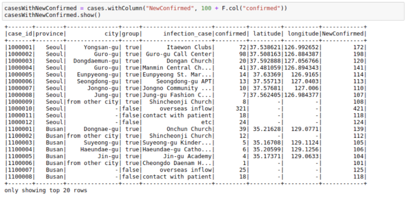

We can also use math functions like the F.exp function:

casesWithExpConfirmed = cases.withColumn("ExpConfirmed", 
F.exp("confirmed"))
casesWithExpConfirmed.show()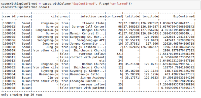

A lot of other functions are provided in this module, which are enough for most simple use cases. You can check out the functions list here.

 

Using Spark UDFs

Sometimes, we want to do complicated things to a column or multiple columns. We can think of this as a map operation on a PySpark DataFrame to a single column or multiple columns. Although Spark SQL functions do solve many use cases when it comes to column creation, I use Spark UDF whenever I need more matured Python functionality.

To use Spark UDFs, we need to use the F.udf function to convert a regular Python function to a Spark UDF. We also need to specify the return type of the function. In this example, the return type is StringType()

import pyspark.sql.functions as F
from pyspark.sql.types import *
def casesHighLow(confirmed):
    if confirmed < 50: 
        return 'low'
    else:
        return 'high'
    
#convert to a UDF Function by passing in the function and return type of function
casesHighLowUDF = F.udf(casesHighLow, StringType())
CasesWithHighLow = cases.withColumn("HighLow", 
casesHighLowUDF("confirmed"))
CasesWithHighLow.show()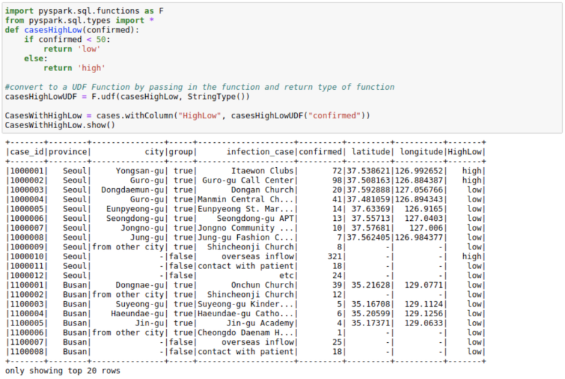

 

Using RDDs

This might seem a little odd, but sometimes, both the Spark UDFs and SQL functions are not enough for a particular use case. I have observed the RDDs being much more performant in some use cases in real life. We might want to use the better partitioning that Spark RDDs offer. Or you may want to use group functions in Spark RDDs.

Whatever the case may be, I find that using RDD to create new columns is pretty useful for people who have experience working with RDDs, which is the basic building block in the Spark ecosystem. Don’t worry much if you don’t understand this, however. It’s just here for completion.

This process makes use of the functionality to convert between Row and Pythondict objects. We convert a row object to a dictionary. We then work with the dictionary as we are used to and convert that dictionary back to row again. This approach might come in handy in a lot of situations.

import math
from pyspark.sql import Row
def rowwise_function(row):
    # convert row to python dictionary:
    row_dict = row.asDict()
    # Add a new key in the dictionary with the new column name and 
value.
    # This might be a big complex function.
    row_dict['expConfirmed'] = float(np.exp(row_dict['confirmed']))
    # convert dict to row back again:
    newrow = Row(**row_dict)
    # return new row
    return newrow
# convert cases dataframe to RDD
cases_rdd = cases.rdd
# apply our function to RDD
cases_rdd_new = cases_rdd.map(lambda row: rowwise_function(row))
# Convert RDD Back to DataFrame
casesNewDf = sqlContext.createDataFrame(cases_rdd_new)
casesNewDf.show()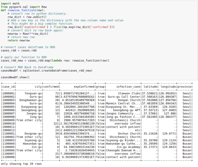

 

Using Pandas UDF

This functionality was introduced in Spark version 2.3.1. It allows the use of Pandas functionality with Spark. I generally use it when I have to run a groupBy operation on a Spark DataFrame or whenever I need to create rolling features and want to use Pandas rolling functions/window functions rather than Spark versions, which we will go through later.

We use the F.pandas_udf decorator. We assume here that the input to the function will be a Pandas DataFrame. And we need to return a Pandas DataFrame in turn from this function.

The only complexity here is that we have to provide a schema for the output DataFrame. We can use the original schema of a DataFrame to create the outSchema.

cases.printSchema()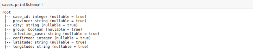

Here, I’m using Pandas UDF to get normalized confirmed cases grouped by infection_case. The main advantage here is that I get to work with Pandas DataFrames in Spark.

from pyspark.sql.types import IntegerType, StringType, DoubleType, BooleanType
from pyspark.sql.types import StructType, StructField

# Declare the schema for the output of our function

outSchema = StructType([StructField('case_id',IntegerType(),True),
                        StructField('province',StringType(),True),
                        StructField('city',StringType(),True),
                        StructField('group',BooleanType(),True),
                        StructField('infection_case',StringType(),True),
                        StructField('confirmed',IntegerType(),True),
                        StructField('latitude',StringType(),True),
                        StructField('longitude',StringType(),True),
                        StructField('normalized_confirmed',DoubleType(),True)
                       ])
# decorate our function with pandas_udf decorator
@F.pandas_udf(outSchema, F.PandasUDFType.GROUPED_MAP)
def subtract_mean(pdf):
    # pdf is a pandas.DataFrame
    v = pdf.confirmed
    v = v - v.mean()
    pdf['normalized_confirmed'] = v
    return pdf

confirmed_groupwise_normalization = cases.groupby("infection_case").apply(subtract_mean)

confirmed_groupwise_normalization.limit(10).toPandas()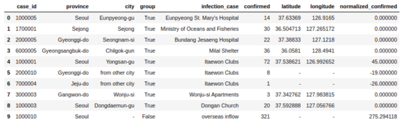

Get Your Data Career GoingHow to Become a Data Analyst From Scratch

 

7. Spark Window Functions

Window functions may make a whole blog post in themselves. Here, however, I will talk about some of the most important window functions available in Spark.

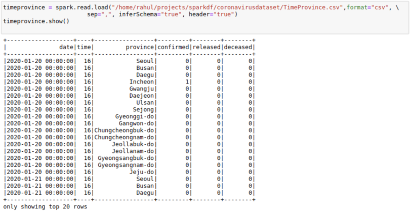
For this, I will also use one more data CSV, which contains dates, as that will help with understanding window functions. I will use the TimeProvince DataFrame, which contains daily case information for each province.

 

Ranking

We can get rank as well as dense_rank on a group using this function. For example, we may want to have a column in our cases table that provides the rank of infection_case based on the number of infection_case in a province. We can do this as follows:

from pyspark.sql.window import Window
windowSpec = 
Window().partitionBy(['province']).orderBy(F.desc('confirmed'))
cases.withColumn("rank",F.rank().over(windowSpec)).show()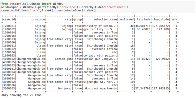

 

Lag Variables

Sometimes, our data science models may need lag-based features. For example, a model might have variables like last week’s price or the sales quantity for the previous day. We can create such features using the lag function with window functions. Here, I am trying to get the confirmed cases seven days before. I’m filtering to show the results as the first few days of coronavirus cases were zeros. You can see here that the lag_7 day feature is shifted by seven days.

from pyspark.sql.window import Window
windowSpec = Window().partitionBy(['province']).orderBy('date')
timeprovinceWithLag = 
timeprovince.withColumn("lag_7",F.lag("confirmed", 
7).over(windowSpec))
timeprovinceWithLag.filter(timeprovinceWithLag.date>'2020-03-
10').show()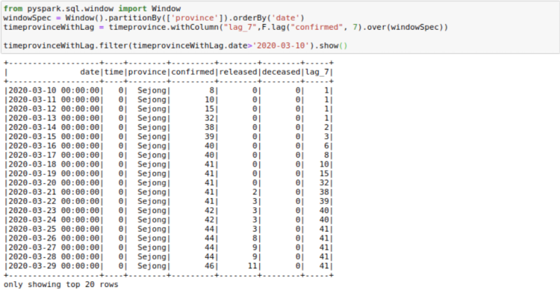

 

Rolling Aggregations

Sometimes, providing rolling averages to our models is helpful. For example, we might want to have a rolling seven-day sales sum/mean as a feature for our sales regression model. Let’s calculate the rolling mean of confirmed cases for the last seven days here. A lot of people are already doing so with this data set to see real trends.

from pyspark.sql.window import Window
windowSpec = 
Window().partitionBy(['province']).orderBy('date').rowsBetween(-6,0)
timeprovinceWithRoll = timeprovince.withColumn("roll_7_confirmed",F.mean("confirmed").over(wi
ndowSpec))
timeprovinceWithRoll.filter(timeprovinceWithLag.date>'2020-03-
10').show()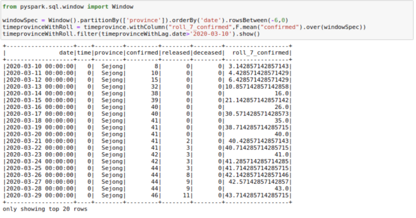

There are a few things here to understand. First is the rowsBetween(-6,0) function that we are using here. This function has a form of rowsBetween(start,end) with both start and end inclusive. Using this, we only look at the past seven days in a particular window including the current_day. Here, zero specifies the current_row and -6 specifies the seventh row previous to current_row. Remember, we count starting from zero.

So, to get roll_7_confirmed for the date March 22, 2020, we look at the confirmed cases for the dates March 16 to March 22, 2020 and take their mean.

If we had used rowsBetween(-7,-1), we would just have looked at the past seven days of data and not the current_day.

We could also find a use for rowsBetween(Window.unboundedPreceding, Window.currentRow) where we take the rows between the first row in a window and the current_row to get running totals. I am calculating cumulative_confirmed here.

from pyspark.sql.window import Window
windowSpec = Window().partitionBy(['province']).orderBy('date').rowsBetween(Window.
unboundedPreceding,Window.currentRow)
timeprovinceWithRoll = timeprovince.withColumn("cumulative_confirmed",F.sum("confirmed").over
(windowSpec))
timeprovinceWithRoll.filter(timeprovinceWithLag.date>'2020-03-
10').show()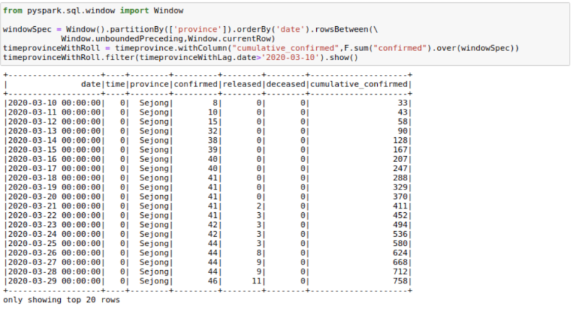

 

8. Pivot DataFrames

Sometimes, we may need to have the DataFrame in flat format. This happens frequently in movie data where we may want to show genres as columns instead of rows. We can use pivot to do this. Here, I am trying to get one row for each date and getting the province names as columns.

pivotedTimeprovince = 
timeprovince.groupBy('date').pivot('province').agg(F.sum('confirmed').
alias('confirmed') , F.sum('released').alias('released'))
pivotedTimeprovince.limit(10).toPandas()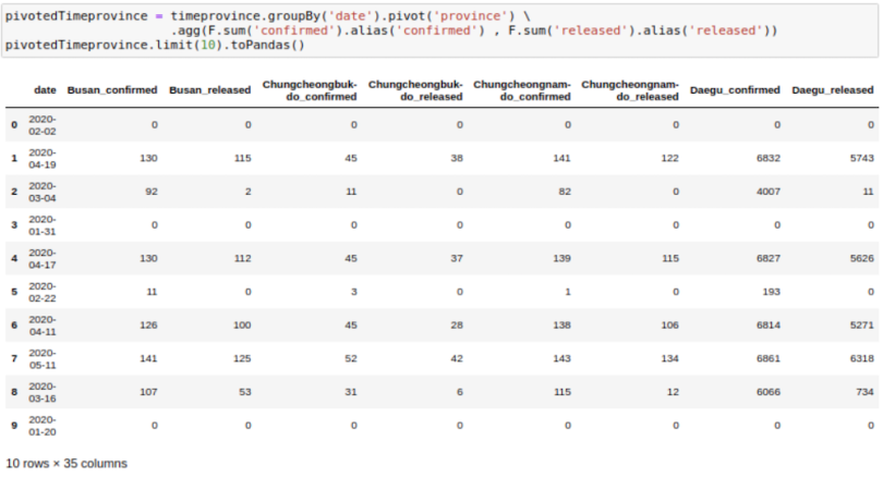

One thing to note here is that we always need to provide an aggregation with the pivot function, even if the data has a single row for a date.

 

9. Unpivot/Stack DataFrames

This is just the opposite of the pivot. Given a pivoted DataFrame like above, can we go back to the original?

Yes, we can. But the way to do so is not that straightforward. For one, we will need to replace - with _ in the column names as it interferes with what we are about to do. We can simply rename the columns:

newColnames = [x.replace("-","_") for x in 
pivotedTimeprovince.columns]
pivotedTimeprovince = pivotedTimeprovince.toDF(*newColnames)

Now, we will need to create an expression which looks like this:

"stack(34, 'Busan_confirmed' , Busan_confirmed,'Busan_released' , Busan_released,'Chungcheongbuk_do_confirmed' ,
.
.
.
'Seoul_released' , Seoul_released,'Ulsan_confirmed' , 
Ulsan_confirmed,'Ulsan_released' , Ulsan_released) as (Type,Value)"

The general format is as follows:

"stack(<cnt of columns you want to put in one column>, 'firstcolname', firstcolname , 'secondcolname' ,secondcolname ......) as (Type, Value)"

It may seem daunting, but we can create such an expression using our programming skills.

expression = ""
cnt=0
for column in pivotedTimeprovince.columns:
    if column!='date':
        cnt +=1
        expression += f"'{column}' , {column},"
expression = f"stack({cnt}, {expression[:-1]}) as (Type,Value)"

And we can unpivot using this:

unpivotedTimeprovince = 
pivotedTimeprovince.select('date',F.expr(exprs))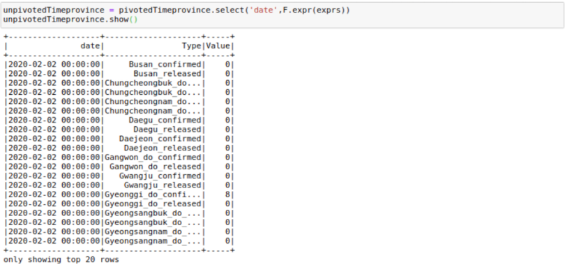

And voila! We’ve got our DataFrame in a vertical format. Quite a few column creations, filters, and join operations are necessary to get exactly the same format as before, but I will not get into those here.

Master Data SciencePublish Your Python Code to PyPI in 5 Simple Steps

 

10. Salting

Sometimes a lot of data may go to a single executor since the same key is assigned for a lot of rows in our data. Salting is another way to manage data skewness.

So, let’s assume we want to do the sum operation when we have skewed keys. We can start by creating the salted key and then doing a double aggregation on that key as the sum of a sum still equals the sum. To understand this, assume we need the sum of confirmed infection_cases on the cases table and assume that the key infection_cases is skewed. We can do the required operation in three steps.

 

Step One: Create a Salting Key

We first create a salting key using a concatenation of the infection_case column and a random_number between zero and nine. In case your key is even more skewed, you can split it into even more than 10 parts.

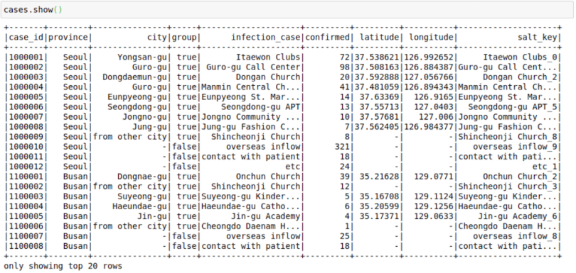
cases = cases.withColumn("salt_key", F.concat(F.col("infection_case"), 
F.lit("_"), F.monotonically_increasing_id() % 10))

This is how the table looks after the operation:

 

Step Two: First Groupby on Salt Key

cases_temp = 
cases.groupBy(["infection_case","salt_key"]).agg(F.sum("confirmed")).s
how()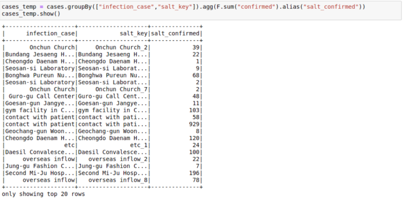

 

3. Second Group On the Original Key

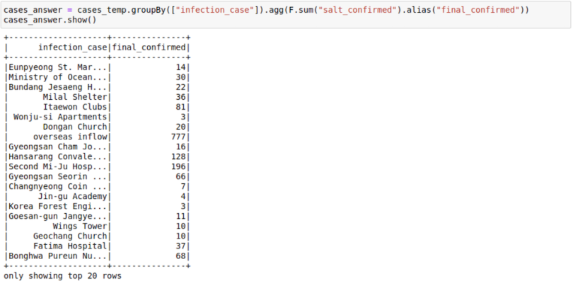
Here, we see how the sum of sum can be used to get the final sum. You can also make use of facts like these:

• Min of min is min
• Max of max is max
• Sum of count is count

You can think about ways in which salting as an idea could be applied to joins too.

 

11. Some More Tips and Tricks for PySpark DataFrames

Finally, here are a few odds and ends to wrap up.

 

Caching

Spark works on the lazy execution principle. What that means is that nothing really gets executed until we use an action function like the .count() on a DataFrame. And if we do a .count function, it generally helps to cache at this step. So, I have made it a point to cache() my DataFrames whenever I do a .count() operation.

df.cache().count()

 

Save and Load From an Intermediate Step

df.write.parquet("data/df.parquet")
df.unpersist()
spark.read.load("data/df.parquet")

When you work with Spark, you will frequently run with memory and storage issues. Although in some cases such issues might be resolved using techniques like broadcasting, salting or cache, sometimes just interrupting the workflow and saving and reloading the whole DataFrame at a crucial step has helped me a lot. This helps Spark to let go of a lot of memory that gets used for storing intermediate shuffle data and unused caches.

 

Repartitioning

You might want to repartition your data if you feel it has been skewed while working with all the transformations and joins. The simplest way to do so is by using this method:

df = df.repartition(1000)

Sometimes you might also want to repartition by a known scheme as it might be used by a certain join or aggregation operation later on. You can use multiple columns to repartition using this:

df = df.repartition('cola', 'colb','colc','cold')

You can get the number of partitions in a DataFrame using this:

df.rdd.getNumPartitions()

You can also check out the distribution of records in a partition by using the glom function. This helps in understanding the skew in the data that happens while working with various transformations.

df.glom().map(len).collect()

 

Reading Parquet File in Local

Sometimes, you might want to read the parquet files in a system where Spark is not available. In such cases, I normally use this code:

from glob import glob
def load_df_from_parquet(parquet_directory):
   df = pd.DataFrame()
   for file in glob(f"{parquet_directory}/*"):
      df = pd.concat([df,pd.read_parquet(file)])
   return df

The Theory Behind the DataWant Better Research Results? Remember Your Priors.

 

Wrapping Up

This was a big article, so congratulations on reaching the end. These are the most common functionalities I end up using in my day-to-day job.

Hopefully, I’ve covered the DataFrame basics well enough to pique your interest and help you get started with Spark. If you want to learn more about how Spark started or RDD basics, take a look at this post

You can find all the code at this GitHub repository where I keep code for all my posts.

Also, if you want to learn more about Spark and Spark DataFrames, I would like to call out the Big Data Specialization on Coursera.