A Deep Dive Into Deep Q-Learning

In part one of this series, I introduced Markov decision processes, the foundation of deep reinforcement learning. Before diving into this article, I recommend you start there. 

In part two, we’ll discuss deep Q-learning, which we use to program AI agents to operate in environments with discrete actions spaces. A discrete action space refers to actions that are specific and well-defined (e.g. moving left or right, up or down).

Atari’s Breakout demonstrates an environment with a discrete action space. The AI agent can move either left or right; the movement in each direction is happening with a certain velocity. 

If the agent can determine the velocity, then it could have continuous action space with an infinite amount of possible actions (including movements with a different velocity). We’ll talk more about this in a bit. 

More From Artem OppermannArtificial Intelligence vs. Machine Learning vs. Deep Learning

Action-Value Function

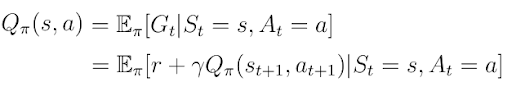
In the last article, I introduced the concept of the action-value function Q(s,a) (equation 1). As a reminder the action-value function is the expected return the AI agent would get by starting in state s, taking action a and then following a policy π.

Note: We can describe the policy π as a strategy of the agent to select certain actions depending on the current state s.

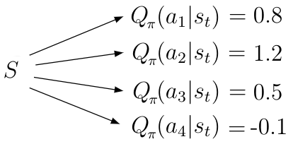
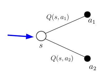
Q(s,a) tells the agent the value (or quality) of a possible action a in a particular state s. Given a state s, the action-value function calculates the quality/value for each possible action a_i in this state as a scalar value (figure 1). Higher quality means a better action with regards to the given objective.

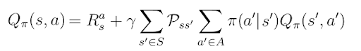
If we execute the expectation operator E in equation 1, we obtain a new form of the action-value function where we’re dealing with probabilities. Pss’ is the transition probability from state s to the next state s’, determined by the environment. π(a’|s’) is the policy or, mathematically speaking, the distribution over all actions given a state s.

Back to BasicsHow AI Teach Themselves Through Deep Reinforcement Learning

Temporal Difference Learning

Our goal in deep Q-learning is to solve the action-value function Q(s,a). Why? If the AI agent knows Q(s,a) then the agent will consider the given objective (like winning a chess game versus a human player or playing Atari’s Breakout) solved because the knowledge of Q(s,a) enables the agent to determine the quality of any possible action in any given state. With that knowledge, the agent could behave accordingly and in perpetuity.

Equation 2 also gives us a recursive solution we can use to calculate Q(s,a). But since we’re considering recursion and dealing with probabilities, using this equation isn’t practical. Instead, we must use the temporal difference (TD) learning algorithm to solve Q(s,a) iteratively.

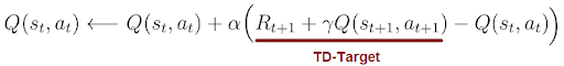
In TD learning we update Q(s,a) for each action a in a state s towards the estimated return R(t+1)+γQ(s(t+1), a(t+1)) (equation 3). The estimated return is also called the TD-target. Performing this update rule iteratively for each state s and action a many times yields correct action-values Q(s,a) for any state — action pair in the environment.

We can summarize the TD-Learning algorithm in the following steps:

• Calculate Q(s_t, a_t) for the action a_t in state s_t

• Go to the next state s_(t+1), take an action a(t+1) there and calculate the valueQ( s_(t+1), a(t+1))

• Use Q( s_(t+1), a(t+1)) and the immediate reward R(t+1) for the action a_t in the last state s_t to calculate the TD-target

• Update previous Q(s_t, a_t) by adding Q(s_t, a_t) to the difference between the TD-target and Q(s_t, a_t), α being the learning rate.

Temporal Difference

Let’s discuss the concept of the TD algorithm in greater detail. In TD-learning we consider the temporal difference of Q(s,a) — the difference between two “versions” of Q(s, a) separated by time once before we take an action a in state s and once after that.

Before taking action

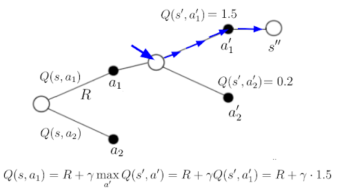
Take a look at figure 2. Assume the AI agent is in state s (blue arrow). In state s, he can take two different actions a_1 and a_2. Based on the calculations from some previous time steps the agent knows the action-values Q(s, a_1) and Q(s, a_2) for the two possible actions in this state.

After Taking Action

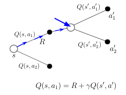
Based on this knowledge, the agent decides to take the action a_1. After taking this action the agent is in the next state s’. For taking the action a_1 he receives the immediate reward R. Being in state s’ the agent can again take two possible actions a’_1 and a’_2 for which he knows the action-values again from some previous calculations.

If you look at the definition of Q(s,a) in equation 1 you’ll recognize that in state s’ we now have new information that we can use to calculate a new value for Q(s, a_1). This information is the immediate reward R received for the last action in the last state and Q(s’,a’) for the action a’ the agent will take in this new state. We can calculate the new value of Q(s, a_1) according to the equation in figure 3. The right side of the equation is also what we call the TD-target. The difference between the TD-target and the old value (or temporal version) of Q(s,a_1) is called temporal difference.

Note: During TD-learning we calculate temporal differences for any possible action-value Q(s,a) and use them to update Q(s,a) at the same time, until Q(s,a) has converged to its true values.

Built In Deep Learning ExpertsThink You Don’t Need Loss Functions in Deep Learning? Think Again.

SARSA

The TD-learning algorithm applied to Q(s,a) is commonly known as the SARSA algorithm (state–action–reward–state–action). SARSA is a good example of the special kind of learning algorithms, also known as on-policy algorithms.

Earlier I introduced the policy π(a|s) as a mapping from state s to action a. One thing that you should remember at this point is that on-policy algorithms use the same policy to obtain the actions for Q(s_t, a_t) as well as the actions for Q(s(t+1), a_(t+1)) in the TD-target. This means we’re following and improving the same policy at the same time.

Q-Learning

We’ve finally arrived at Q-learning. First we must take a look at the second special type of algorithms called off-policy algorithms. As you may already know Q-learning belongs in this category of algorithm, which is distinct from on-policy algorithms such as SARSA.

To understand off-policy algorithms we must introduce the behavior policy µ(a|s). Behavior policy determines the actions a_t~µ(a|s) for Q(s_t,a_t) for all t. In the case of SARSA, the behavior policy would be the policy that we follow and try to optimize at the same time.

In off-policy algorithms we have two different policies, µ(a|s) and π(a|s). µ(a|s) is the behavior and π(a|s) is the target. While we use the behavior policy to calculate Q(s_t, a_t), we use the target policy for the calculation of Q(s_t, a_t) only in the TD-target. (We’ll come back to this in the next section, where we’ll make actual calculations.)

Note: Behavior policy picks actions for all Q(s,a). In contrast, the target policy determines the actions only for TD-target’s calculation.

The algorithm we call the Q-learning algorithm is a special case where the target policy π(a|s) is a greedy w.r.t. Q(s,a), which means that our strategy takes actions which result in the highest values of Q. Following target policy, that yields:

In this case, the target policy is called the greedy policy. Greedy policy means we only pick actions that result in highest Q(s,a) values. We can insert this greedy target policy into the equation for action-values Q(s,a) where we previously followed a random policy π(a|s):

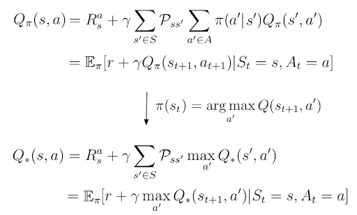
The greedy policy provides us with optimal action-values Q*(s,a) because, by definition, Q*(s,a) is Q(s,a) that follows the policy that maximizes the action-values:

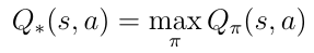
The last line in equation 5 is nothing more than the Bellman optimality equation which we derived in part one of this series. We use this equation as a recursive update rule to estimate the optimal action-value function Q*(s,a).

However, TD-learning remains the best way to find Q*(s,a). With greedy target policy the TD-learning update step for Q(s,a) in equation 3 becomes simpler and looks as follows:

We can summarize the TD-learning algorithm for Q(s,a) with a greedy target policy in the following steps:

• Calculate Q(s_t, a_t) for the action a_t in state s_t

• Go to the next state s_(t+1), take the action a’ that results in highest values of Q and calculate Q( s_(t+1), a’)

• Use Q( s_(t+1), a’) and the immediate reward R for the action a_t in the last state s_t to calculate the TD-target

• Update previous Q(s_t, a_t) by adding Q(s_t, a_t) to the difference between the TD-target and Q(s_t, a_t), α being the learning rate

Consider figure 3 above, where the agent landed in state s’ and knew the action values for the possible actions in that state. Following the greedy target policy, the agent would take the action with the highest action-value (blue path in figure 4). This policy also gives us a new value for Q(s, a_1) (see equation in figure 4 below), which is, by definition, the TD-target.

News You Can UseAI Makes Decisions We Don’t Understand. That’s a Problem.

Deep Q-Learning

We’re finally ready to make use of deep learning. If you look at the updated rule for Q(s,a) you may recognize we don't get any updates if the TD-target and Q(s,a) have the same values. In this case Q(s,a), converges to the true action-values and achieves the goal.

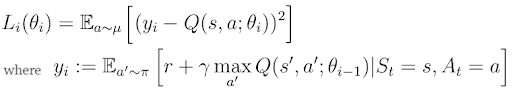
This means our objective is minimizing the distance between the TD-target and Q(s,a), which we can express with the squared error loss function (equation 10). We minimize this loss function by way of usual gradient descent algorithms.

Target and Q-Network

In deep Q-learning, we estimate TD-target y_i and Q(s,a) separately by two different neural networks, often called the target and Q-networks (figure 4). The parameters θ(i-1) (weights, biases) of the target-network correspond to the parameter θ(i) of the Q-network at an earlier point in time. In other words, the target-network parameters are frozen in time and updated after n iterations with the parameters of the Q-network.

Note: Given the current state s, the Q-network calculates the action-values Q(s,a). At the same time the Target-network uses the next state s’ to calculate Q(s’,a) for the TD-target.

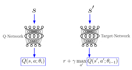
Research shows using two different neural networks for TD-target and Q(s,a) calculation leads to better model stability.

ε-Greedy Policy

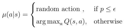
While the target policy π(a|s) remains the greedy policy, the behavior policy µ(a|s) determines the action a_i the AI agent takes, thus which Q(s,a_i) the model must insert into the squared error loss function (calculated by the Q-network).

We typically choose ε-Greedy for behavior policy because with ε-Greedy policy, the agent selects a random action with a fixed probability ε at each time step. If ε has a higher value than a randomly generated number p, 0 ≤ p ≤ 1, the AI agent picks a random action from the action space. Otherwise, the action is chosen greedily according to the leaned action-value Q(s,a):

Choosing ε-Greedy policy as the behavior policy µ solves the dilemma of the exploration/exploitation trade off.

Exploration/Exploitation

Deciding which action to take involves a fundamental choice:

• Exploitation: Make the best decision given the current information

• Exploration: Gather more information, explore possible new paths

In terms of exploitation, the agent takes the best possible action according to the behavior policy µ. But this may result in a problem. There may be another (alternative) action the agent can take that results (long term) in a better path through the sequence of states. However, the agent cannot take this alternative action if we follow the behavior policy. In this case, we exploit the current policy but don’t explore other alternative actions.

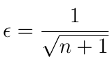
The ε-Greedy policy solves this problem by allowing the AI agent to take random actions from the action-space with a certain probability ε. This is called exploration. Usually, the value of ε decreases over time, according to equation 12. Here n equals the number of iterations. Decreasing ε means that, at the beginning of training, we try to explore more alternative paths but, in the end, we let the policy make decisions on which action to take.

Have You Seen Our Jobs?Check Out These Machine Learning Jobs on Built In

Experience Replay

In the past, the neural network approach to estimate the TD-target and Q(s,a) becomes more stable if the deep Q-learning model implemented experience replay. Experience replay is nothing more than the memory that stores < s, s’, a’, r > tuple, where

• s=state of the AI agent

• a’=action taken in the state s by the agent

• r=immediate reward received in state s for action a’

• s’=next state of the agent after state s

While training the neural network we don’t usually use the most recent < s, s’, a’, r > tuple. Rather, we take random batches of < s, s’, a’, r > from the experience replay to calculate the TD-target, Q(s,a) and apply gradient descent in the end.

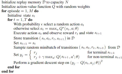
Deep Q-Learning With Experience Replay Pseudo Algorithm

The following pseudo-algorithm implements deep Q-learning with experience replay. All topics we’ve discussed previously are incorporated in this algorithm in the right order, exactly how you would implement it in code.

We use deep Q-learning, a technique of deep reinforcement learning, to program AI agents that can operate in environments with discrete actions spaces. However, deep Q-learning is not without its limitations and flaws. In the next article, we’ll learn about double Q-learning, an improvement on Q-learning that’s even more efficient in programming AI agents for discrete action spaces.

What’s Next?An Introduction to Double Deep Q-Learning