

A Voronoi diagram, also known as a Dirichlet tessellation or Thiessen polygons, is a type of tessellation pattern where points on a plane are divided into exactly n number of cells, each of which enclose a region of the plane that is closest to its respective point.
Voronoi diagrams are everywhere in nature. You’ve likely encountered them thousands of times, but perhaps didn’t know what they were called. Voronoi diagrams are simple, yet they have incredible properties that have applications in fields ranging from cartography, biology, computer science, statistics, archaeology, all the way to architecture and arts.
Voronoi Diagrams Explained
A Voronoi diagram is a type of tessellation pattern in which a number of points scattered on a plane divides in exactly n cells, where each cell encloses a portion of the plane that is closest to each point. Voronoi diagrams can be found in nature (like biological cells and a giraffe’s coat), architecture, art and computer science.
What Is a Voronoi Diagram?
Suppose you have n points scattered on a plane, the Voronoi diagram of those points subdivides the plane in exactly n cells enclosing the portion of the plane that is the closest to each point. This produces a tessellation that completely covers the plane. In the illustration below, I plotted 100 random points and their corresponding Voronoi diagram. As you can see, every point is enclosed in a cell, whose boundaries are equidistant between two or more points. In other words, the area enclosed in the cell is closer to the point in the cell than to any other point.

Where Are Voronoi Patterns Found?
Voronoi patterns can be found in a number of places, including nature, architecture and the arts. Let’s look at some examples.
Voronoi Patterns in Nature
Voronoi diagram patterns are common in nature. From microscopic cells in onion skins to the shell of jackfruits and the coat of giraffes, these patterns are everywhere.
A reason for their omnipresence is that they form efficient shapes. As we mentioned earlier, a Voronoi diagram completely tessellates the plane. All space is used. This is very convenient if you are trying to squeeze as much as possible in a limited space — such as in biological tissues or bee hives. Voronoi diagrams are also a spontaneous pattern whenever something is growing at a uniform growth rate from separate points as in the illustration below. For instance, this explains why giraffes exhibit such a pattern. Giraffe embryos have a scattered distribution of melanin-secreting cells, which is responsible for the dark pigmentation of the giraffe’s spots. Over the course of the gestation these cells release melanin — hence spots radiate outward. A study from researchers Marcelo Walter, Alan Fournier and Menevaux also explores this concept of using Voronoi diagrams to model computer rendering of spots on animal coats.
Voronoi Patterns in Architecture and Arts
Perhaps because of their spontaneous, natural look, or simply because of their mesmerizing randomness, Voronoi patterns have intentionally been implemented in human-made structures. An architectural example is the “Water Cube,” which was built to house water sports during the 2008 Beijing Olympics. The Water Cube’s design features Voronoi-like diagrams on its ceiling and façades, and were chosen because they recall bubbles. This analogy is clear at night, when the entire façade is illuminated in blue and comes alive.
But appreciation for the Voronoi pattern is surely older than this building in China. Guan and Ge ware from the Song dynasty have a distinctive crackled glaze. Ceramics can easily crack during the cooling process, however the crackles from the Guan and Ge ware are different because they are intentional. They were sought after because of their aesthetic qualities. Thanks to the Voronoi-like patterns on their surface, each piece is unique. To date, they are one of the most imitated styles of porcelain.
Voronoi diagrams are also common in graphic arts for creating “abstract” patterns. I think they make excellent background images. For example, I created the thumbnail of this post by generating random points and constructing a Voronoi diagram. Then, I coloured each cell based on the distance of its point from a randomly selected spot in the box. Endless abstract backgrounds images could be generated this way.

Mathematical Definition and Properties of the Voronoi Diagram
So far, we have presented a simple two-dimensional Voronoi diagram. However, the same type of structure can be generalized to an n-dimensional space. Suppose P={p1,p2,…,pm} is a set of m points in our n-dimensional space. Then the space can be partitioned in m Voronoi cells, Vi, containing all points in Rn that are closer to pi than to any other point.

Where the function d(x,y) gives the distance (a) between its two arguments. Typically, the Euclidean distance is used (l2 distance):

However, Voronoi diagrams could be designed using other distance functions. For instance, the equation below shows a Voronoi diagram obtained with the Manhattan or cityblock distance (l1 distance). The Manhattan distance is the distance between two points if you had to follow a regular grid — such as the city blocks of Manhattan. The result is a more “boxy” or rectangle-like Voronoi diagram.

Euclidean distance is the most common distance measure in scientific applications of the Voronoi diagram. It also has the advantage of generating Voronoi cells that are convex. That is to say, if you take any two points within a cell, the line that connects the two points will lie entirely within the cell.
Finally, it should also be noted that Voronoi diagrams are tightly linked with the k-nearest neighbors algorithm (k-NN) — a very popular algorithm in classification, regression and clustering problems. The algorithm uses the k closest examples in the training data set to make value predictions. Since the Voronoi diagrams partition the space in polygons containing the closest points to each seed, the edges of Voronoi cells correspond exactly to the decision boundaries of a simple 1-nearest neighbor problem.
Voronoi Diagrams and Delaunay Triangulation
If you take each of the points from a Voronoi diagram and link it with the points in its neighboring cells, you will obtain a graph called the Delaunay triangulation. In mathematical terms, the Delaunay triangulation is the dual graph of the Voronoi diagram. In the Figure below, a Voronoi diagram (black) and Delaunay triangulation (gray) is plotted from a set of points.

Delaunay triangulation is just as amazing as Voronoi diagrams. As the name suggests, it produces a set of triangles linking our points. These triangles are such that if one were to draw a circle across the vertices of these triangles, there would be no other point inside the circle. Moreover, Delaunay triangulation also has the property of maximizing the smallest angle in the triangles of the triangulation. Hence, Delaunay triangulation tends to avoid triangles with acute angles.
These properties make it very useful in modeling surfaces and objects from a set of points. For instance, the Delaunay triangulation is used to generate meshes for the finite element method, construct 3D models for computer animations and model terrain in geographic information system (GIS) analysis.
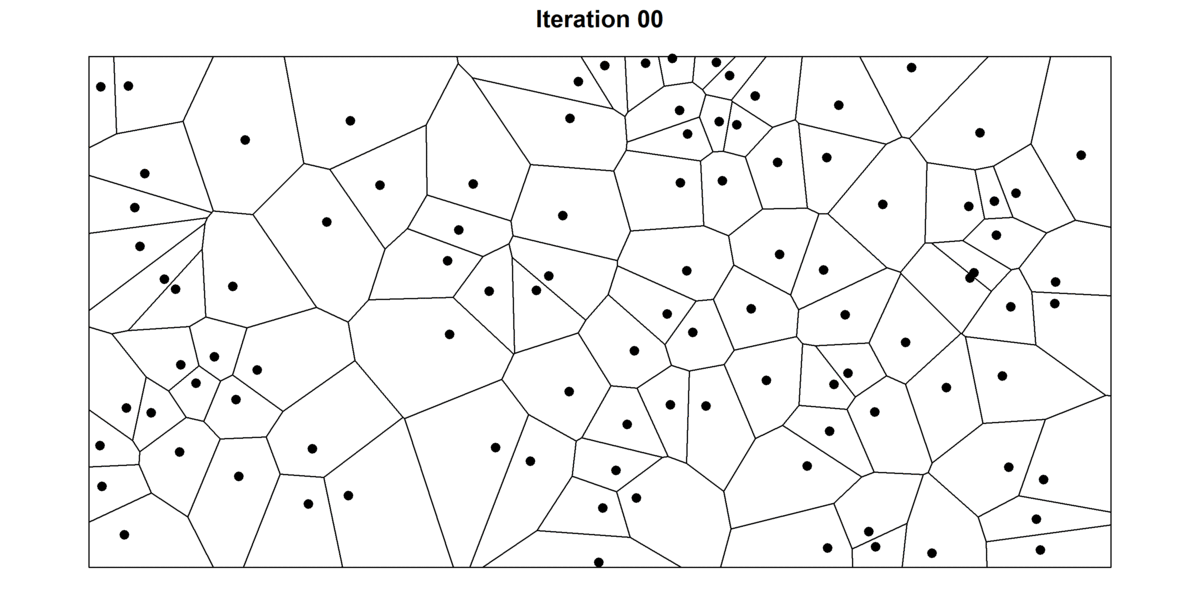
Lloyd’s Relaxation Algorithm in Voronoi Diagrams
Llyod’s algorithm is a useful algorithm related to Voronoi diagrams. The algorithm consists of repeatedly alternating between constructing Voronoi diagrams and finding the centroids (i.e. center of mass) of each cell. At each iteration, the algorithm spaces the points apart and produces more homogeneous Voronoi cells.

After a few iterations, the cells will have a “rounder” aspect, and points will be more evenly distributed. This is illustrated in the figure below, in which I have plotted the first 30 iterations of the Lloyd’s algorithm for a random set of points. For each point, I also record their starting position with a gray hollow circle to better trace the movement of each cell. For a high number of iterations, the diagram tends to converge towards a stable Voronoi diagram in which every seed is also the centroid of the cell — also known as the centroidal Voronoi diagram. Interestingly, in 2D, Voronoi cells will tend to turn into hexagons because they provide the most efficient way of packing shapes in a plane. As any bee building their hive can certify, hexagonal cells have two big advantages:
- They ensure no empty space is left between cells (i.e. it tessellates the plane).
- Hexagons offer the highest ratio between surface and perimeter of the cell. This so-called Honeycomb conjecture took mathematicians 2,000 years to prove.
In data science, Lloyd’s algorithm is the basis of k-means clustering — one of the most popular clustering algorithms. K-means clustering is typically initiated by taking k random “centroids” in space. Then, data points are grouped in k clusters by alternating between assigning data points to the closest “centroid” (this is equivalent to building a Voronoi diagram for the centroid and checking which point are inside the cell) and updating the centroid by calculating the mean of the points inside each cell.
Lloyd’s algorithm is used in a variety of applications. For instance, it is very common in quantization and lossy data compression algorithms, for example the Lloyd-Max algorithm. It is also useful whenever one wants random points that are nicely spaced. For instance, it could be used to generate smooth meshes from the Delaunay triangulation, for dithering images, or as a basis for procedural maps generation in video games.
How to Construct Voronoi Diagrams
One could construct Voronoi diagrams by building each cell one by one. If one extends the bisector of the segments linking every combination of points, it’s possible to obtain the outline of Voronoi cells. However, this technique is quite inefficient. Considering there are 0.5*(n-1)n combinations of points, the complexity of such an algorithm would increase quadratically with the number of points.

More efficient alternatives have been proposed. For example, the Sweep line algorithm builds Voronoi cells progressively by sequentially using binary search tree and priority queue operations.
Another way to construct Voronoi diagrams is to first build Delaunay triangulations. Once the triangulation is obtained, extending the bisectors of the triangle edges leads to the Voronoi diagram. Delaunay triangulation can be obtained without considering every pair of points. For instance, an efficient technique consists of projecting the points on a paraboloid in a higher dimension. The convex hull in higher-dimensional space can be considered to correspond to the Delaunay triangulation in lower-dimensional space, thus, re-projecting the convex hull onto the original space gives the Delaunay triangulation.
There are also different algorithms for computing Voronoi diagrams. New algorithms are continuously being proposed to improve computation efficiency in different circumstances. There are also techniques requiring constant time that generate approximate Voronoi diagrams, such as the jump flooding algorithm.
Frequently Asked Questions
What is a Voronoi diagram?
A Voronoi diagram (also known as a Dirichlet tessellation or Thiessen polygons) is a diagram pattern that divides space into regions (cells) based on proximity to a set of points in a plane, ensuring each region contains all space closer to one point than any other.
What is a Voronoi diagram graph?
A Voronoi diagram graph is a way to represent a Voronoi diagram as a graph, where the regions, edges and vertices of the diagram are treated as nodes and connections. Each site (input point) is connected to neighboring sites whose Voronoi regions share a boundary, thus forming a graph of adjacency. The boundaries between these regions can also be viewed as connections in the graph. The vertices (where three or more regions meet) are points of intersection in the graph structure.
What is a Voronoi diagram used for?
A Voronoi diagram is used to divide space into regions based on proximity to a set of points — each region contains all locations closer to one specific point than to any other. It’s commonly used in fields like geography, computer science, robotics, meteorology, machine learning and more.
Where can Voronoi diagrams be found in real life?
Voronoi diagrams can be found in nature (such as in giraffe coat patterns, onion skin cells, jackfruit shells, biological tissue fibers and bee hives) and architecture and art (such as the Water Cube swimming center in Beijing, China).
What is the relationship between Voronoi diagrams and Delaunay triangulation?
Delaunay triangulation is the dual graph of a Voronoi diagram, connecting points to form triangles that optimize spacing. When a Delauney triangulation is created, extending the bisectors of the triangle edges creates a Voronoi diagram.
What are the pros and cons of Voronoi diagrams?
Some pros of Voronoi diagrams include:
- They quickly show which point (site) is closest to any given location, making proximity analysis easy and efficient.
- They mimic real-world phenomena, making them natural and intuitive.
- They can be applied across many fields, including geography, biology, graphics, machine learning and more.
- They can be constructed fairly efficiently.
Some cons of Voronoi diagrams include:
- They are sensitive to site placement. Even small changes in input points can translate to big changes in the diagram.
- They are computationally complex in dimensions higher than 3D.
- They don’t always account for obstacles or alternative distance metrics.
- They don’t handle weighted influence by default. All sites are treated equally unless you use a weighted variant.


