

In the present era, machines have successfully achieved 99% accuracy in understanding and identifying features and objects in images. We see this daily — smartphones recognizing faces in the camera; the ability to search particular photos with Google Images; scanning text from barcodes or book. All of this is possible thanks to the convolutional neural network (CNN), a specific type of neural network also known as convnet.
If you are a deep learning enthusiast, you've probably already heard about convolutional neural networks, maybe you've even developed a few image classifiers yourself. Modern deep-learning frameworks like Tensorflow and PyTorch make it easy to teach machines about images, however, there are still questions: How does data pass through artificial layers of a neural network? How can a computer learn from it? One way to better explain a convolutional neural network is to use PyTorch. So let's deep dive into CNNs by visualizing an image through every layer.

CONVOLUTIONAL NEURAL NETWORKS Explained
What Is a Convolutional Neural Network?
Before getting started with convolutional neural networks, it's important to understand the workings of a neural network. Neural networks imitate how the human brain solves complex problems and finds patterns in a given set of data. Over the past few years, neural networks have engulfed many machine learning and computer vision algorithms.
The basic model of a neural network consists of neurons organized in different layers. Every neural network has an input and an output layer, with many hidden layers augmented to it based on the complexity of the problem. Once the data is passed through these layers, the neurons learn and identify patterns. This representation of a neural network is called a model. Once the model is trained, we ask the network to make predictions based on the test data. If you are new to neural networks, this article on deep learning with Python is a great place to start.
CNN, on the other hand, is a special type of neural network which works exceptionally well on images. Proposed by Yan LeCun in 1998, convolutional neural networks can identify the number present in a given input image. Other applications using CNNs include speech recognition, image segmentation and text processing. Before convolutional neural networks, multilayer perceptrons (MLP) were used in building image classifiers.
Image classification refers to the task of extracting information classes from a multi-band raster image. Multilayer perceptrons take more time and space for finding information in pictures as every input feature needs to be connected with every neuron in the next layer. CNNs overtook MLPs by using a concept called local connectivity, which involves connecting each neuron to only a local region of the input volume. This minimizes the number of parameters by allowing different parts of the network to specialize in high-level features like a texture or a repeating pattern. Getting confused? No worries. Let’s compare how the images are sent through multilayer perceptrons and convolutional neural networks for a better understanding.
COMPARING MLPS AND CNNS
Considering an MNIST dataset, the total number of entries to the input layer for a multilayer perceptron will be 784 as the input image is of size 28x28=784. The network should be able to predict the number in the given input image, which means the output might belong to any of the following classes ranging from 0–9 (1, 2, 3, 4, 5, 6, 7, 8, 9). In the output layer, we return the class scores, say if the given input is an image having the number “3," then in the output layer the corresponding neuron “3” has a higher class score in comparison to the other neurons. But how many hidden layers do we need to include and how many neurons should be there in each one? Here is an example of a coded MLP:
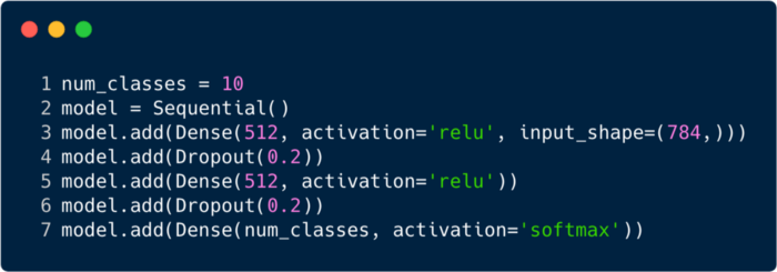
The above code snippet is implemented using a framework called Keras (ignore the syntax for now). It tells us there are 512 neurons in the first hidden layer, which are connected to the input layer of shape 784. The hidden layer is followed by a dropout layer which overcomes the problem of overfitting. The 0.2 indicates there is a 20% probability of not considering the neurons right after the first hidden layer. Again, we added the second hidden layer with the same number of neurons as in the first hidden layer (512), followed by another dropout layer. Finally, we end this set of layers with an output layer comprising 10 classes. This class which has the highest value would be the number predicted by the model.
This is how the multilayer network looks like after all the layers are defined. One disadvantage with this multilayer perceptron is that the connections are complete (fully connected) for the network to learn, which takes more time and space. MLP’s only accept vectors as inputs.

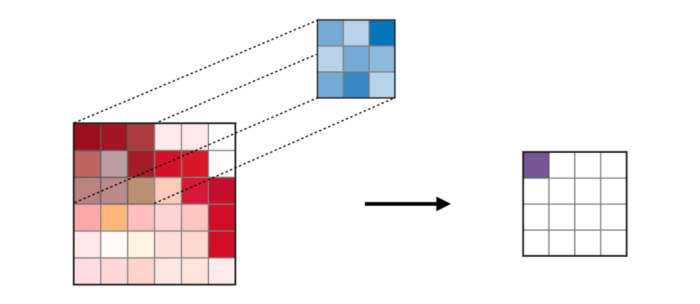
Convolutions don’t use fully connected layers, but sparsely connected layers, that is, they accept matrices as inputs, an advantage over MLPs. The input features are connected to local coded nodes. In MLP, every node is responsible for gaining an understanding of the complete picture. In CNNs, we disintegrate the image into regions (small local areas of pixels). Each hidden node has to report to the output layer, where the output layer combines the received data to find patterns. The image below shows how the layers are connected locally.

Before we can understand how CNNs find information in the pictures, we need to understand how the features are extracted. Convolutional neural networks use different layers and each layer saves the features in the image. For example, consider a picture of a dog. Whenever the network needs to classify a dog, it should identify all the features — eyes, ears, tongue, legs, etc. — and these features are broken down and recognized in the local layers of the network using filters and kernels.
HOW DO COMPUTERS LOOK AT YOUR IMAGE?
Unlike human beings, who understand images by taking snapshots with the eye, computers use a set of pixel values between 0 to 255 to understand a picture. A computer looks at these pixel values and comprehends them. At first glance, it doesn’t know the objects or the colors, it just recognizes pixel values, which is all the image is for a computer.
After analyzing the pixel values, the computer slowly begins to understand if the image is grayscale or color. It knows the difference because grayscale images have only one channel since each pixel represents the intensity of one color. Zero indicates black, and 255 means white, the other variations of black and white, i.e., gray lies in between. Color images, on the other hand, have three channels — red, green and blue. These represent the intensities of three colors (a 3D matrix), and when the values are simultaneously varied, it produces a gives a big set of colors! After figuring out the color properties, a computer recognizes the curves and contours of objects in an image.
This proces can be explored in a convolutional neural network using PyTorch to load the dataset and apply filters to images. Below is the code snippet.
(Find the code on GitHub here)
# Load the libraries
import torch
import numpy as np

from torchvision import datasets
import torchvision.transforms as transforms

# Set the parameters
num_workers = 0
batch_size = 20

# Converting the Images to tensors using Transforms
transform = transforms.ToTensor()

train_data = datasets.MNIST(root='data', train=True,
                                   download=True, transform=transform)
test_data = datasets.MNIST(root='data', train=False,
                                  download=True, transform=transform)

# Loading the Data
train_loader = torch.utils.data.DataLoader(train_data, batch_size=batch_size,
    num_workers=num_workers)
test_loader = torch.utils.data.DataLoader(test_data, batch_size=batch_size,
    num_workers=num_workers)

import matplotlib.pyplot as plt
%matplotlib inline

dataiter = iter(train_loader)
images, labels = dataiter.next()
images = images.numpy()

# Peeking into dataset
fig = plt.figure(figsize=(25, 4))
for image in np.arange(20):
    ax = fig.add_subplot(2, 20/2, image+1, xticks=[], yticks=[])
    ax.imshow(np.squeeze(images[image]), cmap='gray')
    ax.set_title(str(labels[image].item()))

Now let’s see how a single image is fed into the neural network.
(Find the code on GitHub here)
img = np.squeeze(images[7])

fig = plt.figure(figsize = (12,12))
ax = fig.add_subplot(111)
ax.imshow(img, cmap='gray')
width, height = img.shape
thresh = img.max()/2.5
for x in range(width):
    for y in range(height):
        val = round(img[x][y],2) if img[x][y] !=0 else 0
        ax.annotate(str(val), xy=(y,x),
            color='white' if img[x][y]<thresh else 'black')
This is how the number "3" is broken down into pixels. Out of a set of hand-written digits, "3" is randomly chosen wherein the pixel values are shown. In here, ToTensor() normalizes the actual pixel values (0–255) and restricts them to range from 0 to 1. Why? Because, it makes the computations in the later sections easier, either in interpreting the images or finding the common patterns existing in them.
BUILDING YOUR OWN FILTER
In convolutional neural networks, the pixel information in an image is filtered. Why do we need a filter at all? Much like a child, a computer needs to go through the learning process of understanding images. Thankfully, this doesn't take years to do! A computer does this by learning from scratch and then proceeding its way to the whole. Therefore, a network must initially know all the crude parts in an image like the edges, the contours, and the other low-level features. Once these are detected, the computer can then tackle more complex functions. In a nutshell, low-level features must first be extracted, then the middle-level features, followed by the high-level ones. Filters provide a way of extracting that information.
The low-level features can be extracted with a particular filter, which is also a set of pixel values, similar to an image. It can be understood as the weights which connect layers in a CNN. These weights or filters are multiplied with the inputs to arrive at the intermediate images, which depict the partial understanding of the image by a computer. Later, these byproducts are then multiplied with a few more filters to expand the view. This process, along with the detection of features, continues until the computer understands what it's looking at.
There are a lot of filters you can use depending on what you need to do. You might want to blur, sharpen, darken, do edge detection, etc. — all are filters.
Let’s look at a few code snippets to understand the functionalities of filters.


This is how the image looks once the filter is applied. In this case, we’ve used a Sobel filter.
THE COMPLETE CNNS
So far we've seen how filters are used to extract features from images, but to complete the entire convolutional neural network we need to understand the layers we use to design it. The layers used in CNNs are called:
- Convolutional layer
- Pooling layer
- Fully connected layer
Using these three layers, a convolutional image classifier looks like this:

Now let’s see what each layer does:
Convolutional Layer — The convolution layer (CONV) uses filters that perform convolution operations while scanning the input image with respect to its dimensions. Its hyperparameters include the filter size, which can be 2x2, 3x3, 4x4, 5x5 (but not restricted to these alone), and stride (S). The resulting output (O) is called the feature map or activation map and has all the features computed using the input layers and filters. The image below depicts the generation of feature maps when convolution is applied:
Pooling Layer — The pooling layer (POOL) is used for downsampling of the features and is typically applied after a convolution layer. The two types of pooling operations are called max and average pooling, where the maximum and average value of features is taken, respectively. Below, depicts the working of pooling operations:


Fully Connected Layers — The fully connected layer (FC) operates on a flattened input where each input is connected to all the neurons. These are usually used at the end of the network to connect the hidden layers to the output layer, which helps in optimizing the class scores.

VISUALIZING CNNS IN PYTORCH
Now that we have a better understanding of how CNNs function, let’s now implement one using Facebook’s PyTorch framework.
Step 1: Load an input image that should be sent through the network. We'll use Numpy and OpenCV.
(Find the code on GitHub here)
import cv2
import matplotlib.pyplot as plt
%matplotlib inline
img_path = 'dog.jpg'
bgr_img = cv2.imread(img_path)
gray_img = cv2.cvtColor(bgr_img, cv2.COLOR_BGR2GRAY)

# Normalise
gray_img = gray_img.astype("float32")/255
plt.imshow(gray_img, cmap='gray')
plt.show()
Step 2: Visualize the filters to get a better picture of which ones we will be using.
(View the code on GitHub here)
import numpy as np
filter_vals = np.array([
  [-1, -1, 1, 1],
  [-1, -1, 1, 1],
  [-1, -1, 1, 1],
  [-1, -1, 1, 1]
])

print('Filter shape: ', filter_vals.shape)

# Defining the Filters

filter_1 = filter_vals
filter_2 = -filter_1
filter_3 = filter_1.T
filter_4 = -filter_3
filters = np.array([filter_1, filter_2, filter_3, filter_4])

# Check the Filters
fig = plt.figure(figsize=(10, 5))
for i in range(4):
    ax = fig.add_subplot(1, 4, i+1, xticks=[], yticks=[])
    ax.imshow(filters[i], cmap='gray')
    ax.set_title('Filter %s' % str(i+1))
    width, height = filters[i].shape
    for x in range(width):
        for y in range(height):
            ax.annotate(str(filters[i][x][y]), xy=(y,x),
                        color='white' if filters[i][x][y]<0 else 'black')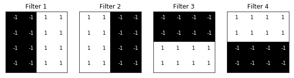
Step 3: Define the CNN. This CNN has a convolutional layer and a max pool layer, and the weights are initialized using the filters depicted above:
(View the code on GitHub here)
import torch
import torch.nn as nn
import torch.nn.functional as F


class Net(nn.Module):

    def __init__(self, weight):
        super(Net, self).__init__()
        # initializes the weights of the convolutional layer to be the weights of the 4 defined filters
        k_height, k_width = weight.shape[2:]
        # assumes there are 4 grayscale filters
        self.conv = nn.Conv2d(1, 4, kernel_size=(k_height, k_width), bias=False)
        # initializes the weights of the convolutional layer
        self.conv.weight = torch.nn.Parameter(weight)
        # define a pooling layer
        self.pool = nn.MaxPool2d(2, 2)

    def forward(self, x):
        # calculates the output of a convolutional layer
        # pre- and post-activation
        conv_x = self.conv(x)
        activated_x = F.relu(conv_x)

        # applies pooling layer
        pooled_x = self.pool(activated_x)

        # returns all layers
        return conv_x, activated_x, pooled_x

# instantiate the model and set the weights
weight = torch.from_numpy(filters).unsqueeze(1).type(torch.FloatTensor)
model = Net(weight)

# print out the layer in the network
print(model)
Net(
(conv): Conv2d(1, 4, kernel_size=(4, 4), stride=(1, 1), bias=False)
(pool): MaxPool2d(kernel_size=2, stride=2, padding=0, dilation=1, ceil_mode=False)
)Step 4: Visualize the filters. Here is a quick glance at the filters being used.
(View the code on GitHub here)
def viz_layer(layer, n_filters= 4):
    fig = plt.figure(figsize=(20, 20))

    for i in range(n_filters):
        ax = fig.add_subplot(1, n_filters, i+1)
        ax.imshow(np.squeeze(layer[0,i].data.numpy()), cmap='gray')
        ax.set_title('Output %s' % str(i+1))

fig = plt.figure(figsize=(12, 6))
fig.subplots_adjust(left=0, right=1.5, bottom=0.8, top=1, hspace=0.05, wspace=0.05)
for i in range(4):
    ax = fig.add_subplot(1, 4, i+1, xticks=[], yticks=[])
    ax.imshow(filters[i], cmap='gray')
    ax.set_title('Filter %s' % str(i+1))


gray_img_tensor = torch.from_numpy(gray_img).unsqueeze(0).unsqueeze(1)
Filters:

Step 5: Filter outputs across the layers. Images that are outputted in the CONV and POOL layer are shown below.
viz_layer(activated_layer)
viz_layer(pooled_layer)
Conv Layers

Pooling Layers

References : CS230 CNNs.
Find the code used for this article here.


