Understanding and Building Neural Network (NN) Models

A neural network is a series of algorithms that endeavors to recognize underlying relationships in a set of data through a process that mimics the way the human brain operates. In that sense, neural networks refer to systems of neurons, either organic or artificial in nature. Neural networks can adapt to a changing input, so the network generates the best possible result without needing to redesign the output criteria.

 

Why Do We Need Neural Networks?

Why do we need yet another learning algorithm? The question is relevant. We already have a lot of learning algorithms like linear regression, logistic regression, decision trees and random forests, etc. I’ll show you a situation in which we have to deal with a complex, non-linear hypothesis.

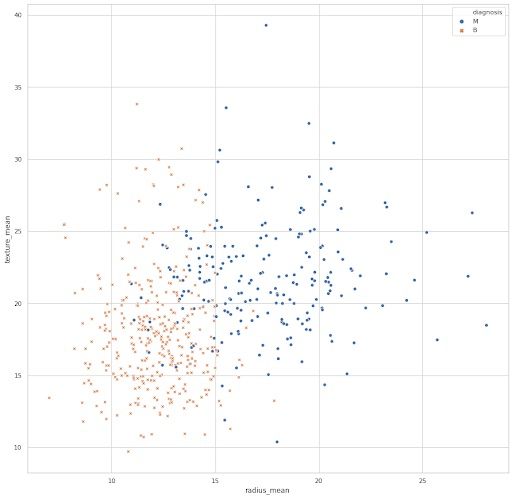
The above plot is obtained from the Breast Cancer Wisconsin data set. I have plotted two of the features, mean radius and mean texture, to gain some information about whether the tumor is malignant (M, represented by blue dots) or benign (B, represented by an orange x).

This is a supervised learning classification problem. If we are to apply logistic regression to this problem, the hypothesis would look like this:

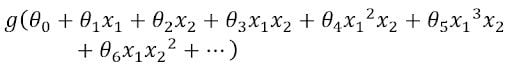
We can see that there are a lot of non-linear features. In this equation, g is the sigmoid function. If we perform logistic regression with such a hypothesis, then we might get a boundary — an extremely curvy one — separating the malignant and benign tumors.

But this is effective only when we’re considering two features. But this data set contains 30 features. If we were to include only the quadratic terms in the hypothesis, we will still have hundreds of non-linear features. The number of quadratic features generated will be to the order of O(n²), where n is the number of features (30). We may end up overfitting the data set. It’s also computationally expensive to work with that many features.

This is if we’re only using quadratic terms. Don’t even try to imagine the number of cubic terms generated in a similar manner.

Enter neural networks.

Model Representation

The NN that is implemented in the computer is called an artificial neural network (ANN), as they simulate the neurons present in the brain. The neurons are responsible for all of the actions voluntarily and involuntarily happening in our bodies. They transmit signals to and from the brain.

More on Machine LearningK-Nearest Neighbor Algorithm: An Introduction

What Is a Neuron Model

First, we will model a neuron as a simple logistic unit.

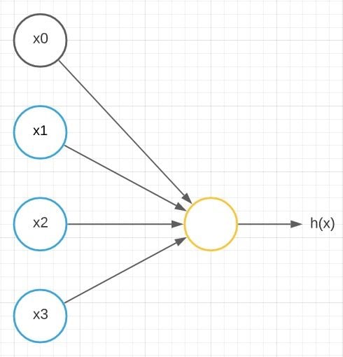
Here x1 , x2 and x3 are the input nodes in blue color. The orange-colored node is the output node outputting h(x). Here’s what I mean by h(x):

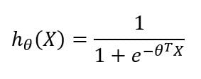
In that equation, x and θ are:

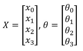
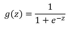
This is a simplified model for the vast range of computations that the neuron completes. It gets input x1, x2 and x3 and outputs a value h(x). The x0 node, which is called the bias unit or bias neuron, is not usually represented pictorially. The above neuron network has a sigmoid (logistic) activation function. The term activation function refers to the non-linearity g(z):

 

What Is a Neural Network?

The above model represents a single neuron. A neural network is a group of these neurons strung together.

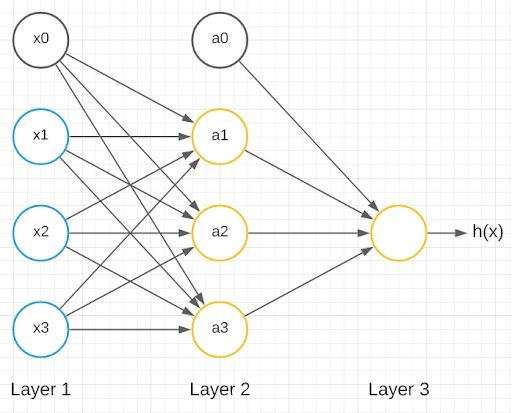
We have inputs x1, x2 and x3 as inputs and x0 as a bias unit. We also have three neurons in the next layer: a1, a2 and a3 with a0 as the bias unit. The last layer has only one neuron, which gives the output. Layer one is called the input layer, layer three is called the output layer and layer two is called the hidden layer. Any layer that isn’t the input layer or the output layer is called the hidden layer.

Let’s delve into the computational steps represented by this diagram:

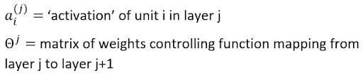
Activation stands for the value computed by, or outputted by, a specific neuron. A neural network is parameterized by the matrix of weights.

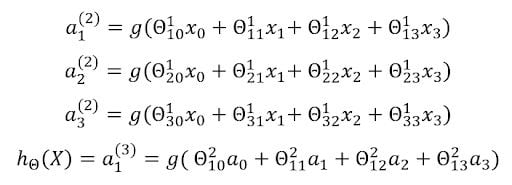
The corresponding weights form the weight matrix, which are multiplied with the inputs and then given as an input to the activation function, here, the sigmoid function, to get the output of the specific neuron. There are three outputs from the three neurons in the hidden layer, and one output from the neuron in the output layer.

If a network has n units in layer j, m units in layer j+1, then the weight matrix corresponding to the layers j and j+1 will be of the dimensions m X(n+1).

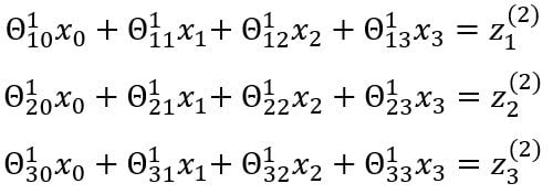
The entire process of multiplying the weights with the inputs and applying the activations function to get the outputs is called forward propagation. The notations can be further simplified:

 

Vectorized Implementation

Instead of representing the above model with individual equations for the outputs of each neuron, we can represent them in the form of a vector.

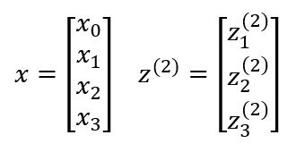
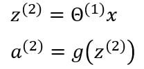
x is the input vector and includes three inputs x1, x2, x3, and a bias unit x0 whose value is mostly equal to one. z is the vector containing the linear products of input with the weight matrix. Forward propagation can be written as:

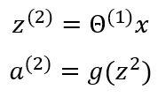
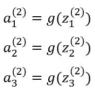
The activation function g applies the sigmoid function element-wise to each of the elements in vector z . We can also denote the input vector as the output of the first layer.

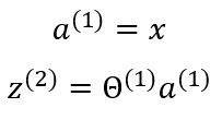
In the above model, there is a bias unit present in the hidden layer. So, we need to add the bias to the output vector of the hidden layer.

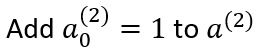
The final output of the output layer is given by:

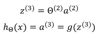
This process is called forward propagation because we start with the input layer and compute the outputs of the hidden layer and then we forward propagate that to compute the activations of the final output layer.

There is no limit to the number of neurons in each layer or the number of layers. We can model a neural network according to our needs and then map the inputs and outputs with suitable weights and activation functions. If there is more than one hidden layer in a neural network, then it’s called a deep neural network.

Now that we know how a neural network calculates its output, the question becomes: How do we train a NN to output the desired values? We had the gradient descent algorithm in linear and logistic regression, which modifies the values of the parameters in order to get the desired output. How does one do that in a neural network?

More on Machine LearningWhat Is Machine Learning and How Does It Work?

 

What Is Backpropagation?

We use the backpropagation algorithm in a NN to compute the gradient, which will allow us to modify the weight matrices discussed above to get the desired output. This is the most important part of NN, and it’s where the model gets trained on the given data. We will discuss the backpropagation algorithm using the same model used above.

The cost function of logistic regression is:

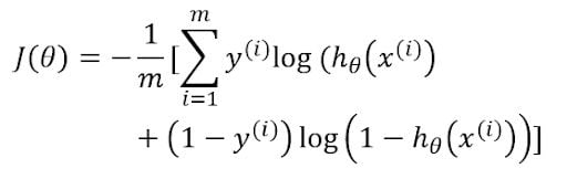
The cost function of the above NN has a sigmoid activation function similar to that of logistic regression. h(x) would be the output of the neuron in the output layer. y is the desired output.

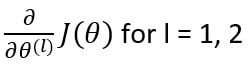
The first step of backpropagation would be to calculate the total cost from the cost function. Our main objective is to change the corresponding weights so that we can minimize this cost. For this, we need to find the gradient of cost with respect to each of the weight matrices. Since we have two weight matrices, the gradients will be:

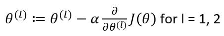
After identifying the gradients, we will update the weight matrices as:

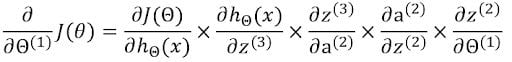
Now to find the gradients, we will use the chain rule of differentiation. 

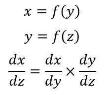
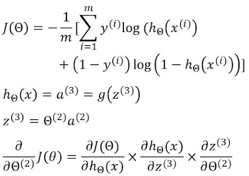
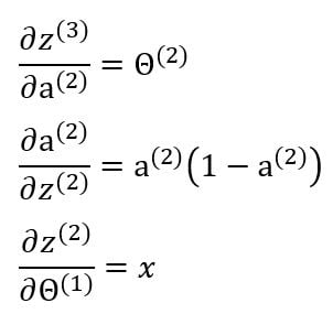
Now we have to find the individual terms in the chain rule.

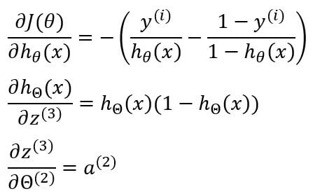
Multiplying all of them together gives us the gradient of cost with respect to the corresponding weight matrix.

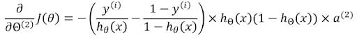
The gradient of cost with respect to the first weight matrix can also be further calculated through this equation:

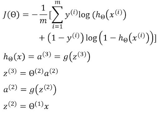
Therefore, the gradient will be:

Individual values are calculated in a similar way. The first two terms are already calculated.

Multiplying them all together gives us the gradient of cost with respect to the weight matrix.

Thus, updating both the weight matrices simultaneously, we’ll get an equation that looks like this:

This completes one iteration of our backpropagation. A set of forward propagation and backpropagation is called an epoch. One epoch is when an entire data set is passed forward and backwards through the neural network once.

Now, let’s discuss the specifics of a neural network.

 

What Is Zero Initialization?

When it comes to training a neural network, weight matrices are the most important part. We need to initialize the weight matrices to a value to perform forward propagation, and the backpropagation to update the initialized weights. What if we initialized all the weights in the NN to zero?

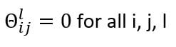
All the activations of the second layer will be equal. Since the gradients of cost with respect to the weights are dependent on the activations, they will be equal, too. While updating the weights after an epoch, the weights will remain the same, as they are initially equal and the gradients are also equal.

This will result in all the neurons computing the same features, thereby outputting a redundant value and preventing the NN from learning. Therefore, random initialization is done to the parameters.

 

How to Train and Model a Neural Network 

The following are the steps involved in modeling and training a neural network.

1. Model the input layer according to the no. of input features.
2. Model the output layer according to the no. of classes in the output.
3. Model the number of hidden layers and the no. of neurons in the hidden layers optimally.
4. Randomly initialize weights.
5. Implement forward propagation to get h(x) for any x.
6. Implement code to compute cost function J.
7. Implement backpropagation to compute the gradient of cost with respect to weights.
8. Update the values of weights.
9. Perform steps five-through-nine recursively to minimize the cost J by modifying the weights after each epoch.

Become a Machine Learning ExpertWhat Is Machine Learning?

 

Building and Training a Neural Network Model From Scratch

There are various libraries available for modeling and training a neural network, but to understand the exact working mechanism of it, we must build it from scratch at-least once. However, we will be using libraries from TensorFlow-Keras (tf.keras) and scikit-learn (sklearn) to cross-verify our model.

I will use  the breast cancer data set from the University of California, Irvine, Machine Learning Repository. After importing the necessary libraries and data into a pandas DataFrame, you’ll see that there are 32 features and 569 data points in each. Each of the features contains information about a tumor found in a patient. The task is to classify the tumors into “malignant” or “benign” based on these features. The target variable is found to be diagnosis .

Since the feature id has unique entries for all 569 cases, it was set as the index of the data frame. While also searching for missing values, you’ll see that a feature named Unnamed: 32 had 100 percent missing values, causing this feature to be dropped. All the other features were found to be numeric features.

On checking for the unique values in the target variable, array(['M', 'B'], dtype=object), there are two classes in the output: M for malignant and B for benign. These were replaced with 0 for M and 1 for B.

Now that we have cleaned our data set, we are ready to divide it into train and test data. The sklearn’s train_test_split is used to divide 80 percent of the data into train data, and the remaining 20 percent into test data.

After the division, both the train and test inputs are scaled using the StandardScaler from sklearn. Take care to fit the scaler only on the train data and not the test data. Then transform both train and test data using the same classifier to avoid data leakage.

Next we’ll model our neural network. We are creating a class called NeuralNet that has all the required functions. I am pasting the code here, as it is the most important part of our discussion.

class NeuralNet():
    def __init__(self, layers = [30, 14, 1], learning_rate = 0.001, iterations = 100):
        self.params = {}
        self.learning_rate = learning_rate
        self.iterations = iterations
        self.cost = []
        self.sample_size = None
        self.layers = layers
        self.X = None
        self.Y = None
    def init_weights(self):
        np.random.seed(1)
        self.params['theta_1'] = np.random.randn(self.layers[0], self.layers[1])
        self.params['b1'] = np.random.randn(self.layers[1],)
        self.params['theta_2'] = np.random.randn(self.layers[1], self.layers[2])
        self.params['b2'] = np.random.randn(self.layers[2],)
    def sigmoid(self,z):
        return 1.0/(1.0 + np.exp(-z))
    def cost_fn(self, y, h):
        m = len(y)
        cost = (-1/m) * (np.sum(np.multiply(np.log(h), y) + np.multiply((1-y), np.log(1-h))))
        return cost
    def forward_prop(self):
        Z1 = self.X.dot(self.params['theta_1']) + self.params['b1']
        A1 = self.sigmoid(Z1)
        Z2 = A1.dot(self.params['theta_2']) + self.params['b2']
        h = self.sigmoid(Z2)
        cost = self.cost_fn(self.Y, h)
        self.params['Z1'] = Z1
        self.params['Z2'] = Z2
        self.params['A1'] = A1
        return h, cost
    def back_propagation(self, h):
        diff_J_wrt_h = -(np.divide(self.Y, h) - np.divide((1 - self.Y), (1 - h)))
        diff_h_wrt_Z2 = h * (1 - h)
        diff_J_wrt_Z2 = diff_J_wrt_h * diff_h_wrt_Z2
        diff_J_wrt_A1 = diff_J_wrt_Z2.dot(self.params['theta_2'].T)
        diff_J_wrt_theta_2 = self.params['A1'].T.dot(diff_J_wrt_Z2)
        diff_J_wrt_b2 = np.sum(diff_J_wrt_Z2, axis = 0)
        diff_J_wrt_Z1 = diff_J_wrt_A1 * (self.params['A1'] * ((1-self.params['A1'])))
        diff_J_wrt_theta_1 = self.X.T.dot(diff_J_wrt_Z1)
        diff_J_wrt_b1 = np.sum(diff_J_wrt_Z1, axis = 0)
        self.params['theta_1'] = self.params['theta_1'] - self.learning_rate * diff_J_wrt_theta_1
        self.params['theta_2'] = self.params['theta_2'] - self.learning_rate * diff_J_wrt_theta_2
        self.params['b1'] = self.params['b1'] - self.learning_rate * diff_J_wrt_b1
        self.params['b2'] = self.params['b2'] - self.learning_rate * diff_J_wrt_b2
    def fit(self, X, Y):
        self.X = X
        self.Y = Y
        self.init_weights()
        for i in range(self.iterations):
            h, cost = self.forward_prop()
            self.back_propagation(h)
            self.cost.append(cost)
    def predict(self, X):
        Z1 = X.dot(self.params['theta_1']) + self.params['b1']
        A1 = self.sigmoid(Z1)
        Z2 = A1.dot(self.params['theta_2']) + self.params['b2']
        pred = self.sigmoid(Z2)
        return np.round(pred)
    def acc(self, y, h):
        acc = (sum(y == h) / len(y) * 100)
        return acc
    def plot_cost(self):
        fig = plt.figure(figsize = (10,10))
        plt.plot(self.cost)
        plt.xlabel('No. of iterations')
        plt.ylabel('Logistic Cost')
        plt.show()

There are a total of three layers in the model. The first layer is the input layer and has 30 neurons for each of the 30 inputs. The second layer is the hidden layer, and it contains 14 neurons by default. The third layer is the output layer, and since we have two classes, 0 and 1, we require only one neuron in the output layer. The default learning rate is set as 0.001, and the number of iterations or epochs is 100.

Remember, there is a huge difference between the terms epoch and iterations. Consider a dataset of 2,000 data points. We are dividing the data into batches of 500 data points and then training the model on each batch. The number of batches to be trained for the entire data set to be trained once is called iterations. Here, the number of iterations is four. The number of times the entire data set undergoes a cycle of forward propagation and backpropagation is called epochs. Since the data above is not divided into batches, iteration and epochs will be the same.

The weights are initialized randomly. The bias weight is not added with the main input weights, it is maintained separately.

Then the sigmoid activation function and cost function of the neural network are defined. The cost function takes in the predicted output and the actual output as input, and calculates the cost.

The forward propagation function is then defined. The activations of the input layer is calculated and passed on as input to the output layer. All the parameters are stored in a dictionary with suitable labels.

The backpropagation function is defined. It takes in the predicted output to perform backpropagation using the stored parameter values. The gradients are calculated as we discussed above and the weights are updated in the end.

The fit function takes in the input x and desired output y. It calls the weight initialization, forward propagation and backpropagation function in that order and trains the model. The predict function is used to predict the output of the test set. The accuracy function can be used to test the performance of the model. There is also a function available for plotting the cost function vs epochs.

We first train the model by fitting the train data that we extracted from the entire data set.

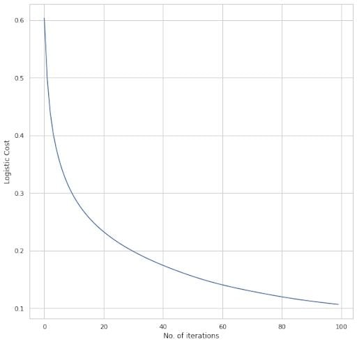
We can see that the total cost is exponentially decreasing as we recursively train the model. The train and test accuracy is found to be Train accuracy: [97.14285714] Test accuracy: [97.36842105]. 

The number of features available ensures we get such a high rate of accuracy. As more information regarding the target variable is available, the model accuracy increases. The above plot and metrics correspond to the default values.

Now, let’s change the default values a bit. The number of neurons in the hidden layer is increased from 14 to 20. The learning rate is decreased from 0.001 to 0.01. The number of iterations has increased from 100 to 500. 

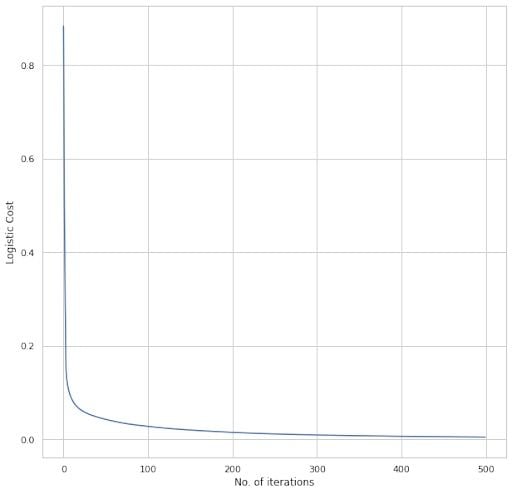
We can see that the cost decreased to somewhere around 0.1 and then reduced gradually to almost zero. The final cost value after 500 iterations is less than the previous case. The train and test accuracies areTrain accuracy: [100.] Test accuracy: [97.36842105].

We can see that the train accuracy reached 100 percent and the test accuracy remained the same.

 

How to Cross-Verify Your Neural Network Model on Sklearn and TF.Keras

For further verification, we’ll use two of the libraries associated with neural networks

 

Sklearn

We will be using sklearn’s MLPClassifier for modeling a neural network, training and testing it. The same parameters used above are being used here. There is one hidden layer consisting of 14 neurons. The learning rate is set as 0.001 and number of iterations as 100.

The train and test accuracies are: 

• Train accuracy = 97.8021978021978 
• Test accuracy = 97.36842105263158

We can see that the train accuracy has increased a bit, and the test accuracy has remained the same. This conveys that our model is in line with the sklearn model.

 

Tensorflow-Keras

We will be modeling a sequential model using tf.keras. It contains two dense layers apart from the input layer. The hidden dense layer consists of 14 neurons, and the output dense layer consists of one neuron. The learning rate is set as 0.001 and binary cross-entropy loss is used. The number of epochs is set as 100. The train and test accuracies are:

• Train accuracy = 98.90109896659851
• Test accuracy = 98.24561476707458

We can see that both the train and test accuracies have increased a bit. The reason for this might be a well-optimized backpropagation algorithm, which helps the model achieve higher accuracies in a fewer  number of iterations.

The tf.keras and sklearn models excels our model in the case of training time. When inputting data that has millions of data-points, the model that we built may take a lot of time to converge or reach acceptable accuracy levels. Whereas, due to the optimization techniques employed in the tf.keras and sklearn models, they may converge faster.