PCA Using Python: A Tutorial

While you can speed up the fitting of a machine learning algorithm by changing the optimization algorithm, a more common way to speed up the algorithm is to use principal component analysis (PCA). If your learning algorithm is too slow because the input dimension is too high, then using PCA to speed it up can be a reasonable choice. This is probably the most common application of PCA. Another common application of PCA is for data visualization.

To understand the value of using PCA for data visualization, the first part of this tutorial post goes over a basic visualization of the Iris data set after applying PCA. The second part, explores how to use PCA to speed up a machine learning algorithm (logistic regression) on the Modified National Institute of Standards and Technology (MNIST) data set.

With that, let’s get started. 

PCA for Data Visualization

For a lot of machine learning applications, it helps to visualize your data. Visualizing two- or three-dimensional data is not that challenging. However, even the Iris data set used in this part of the tutorial is four-dimensional. You can use PCA to reduce that four-dimensional data into two or three dimensions so that you can plot, and hopefully, understand the data better.

More on Data ScienceHowt o Use a Z-Table and Create Your Own

Step 1: Load the Iris Data Set

The iris data set comes with scikit-learn and doesn’t require you to download any files from some external websites. The code below will load the Iris data set.

import pandas as pd

url = "https://archive.ics.uci.edu/ml/machine-learning-databases/iris/iris.data"

# load dataset into Pandas DataFrame
df = pd.read_csv(url, names=['sepal length','sepal width','petal length','petal width','target'])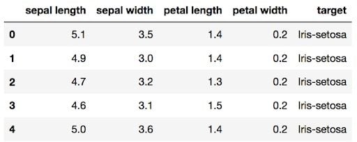

Step 2: Standardize the Data

PCA is affected by scale, so you need to scale the features in your data before applying PCA. Use StandardScaler to help you standardize the data set’s features onto unit scale (mean = 0 and variance = 1), which is a requirement for the optimal performance of many machine learning algorithms. If you don’t scale your data, it can have a negative effect on your algorithm. 

from sklearn.preprocessing import StandardScaler

features = ['sepal length', 'sepal width', 'petal length', 'petal width']

# Separating out the features
x = df.loc[:, features].values

# Separating out the target
y = df.loc[:,['target']].values

# Standardizing the features
x = StandardScaler().fit_transform(x)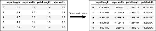

Step 3: PCA Projection to 2D

The original data has four columns (sepal length, sepal width, petal length and petal width). In this section, the code projects the original data, which is four-dimensional, into two dimensions. After dimensionality reduction, there usually isn’t a particular meaning assigned to each principal component. The new components are just the two main dimensions of variation.

from sklearn.decomposition import PCA

pca = PCA(n_components=2)

principalComponents = pca.fit_transform(x)

principalDf = pd.DataFrame(data = principalComponents
             , columns = ['principal component 1', 'principal component 2'])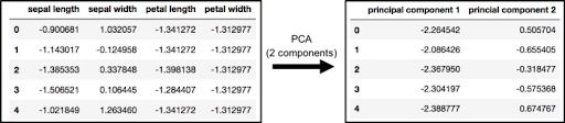

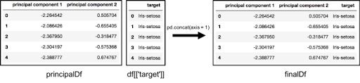
finalDf = pd.concat([principalDf, df[['target']]], axis = 1)

Concatenating DataFrame along axis = 1. finalDf is the final DataFrame before plotting the data.

Step 4: Visualize 2D Projection

This section is just plotting two-dimensional data. Notice on the graph below that the classes seem well separated from each other.

fig = plt.figure(figsize = (8,8))
ax = fig.add_subplot(1,1,1) 
ax.set_xlabel('Principal Component 1', fontsize = 15)
ax.set_ylabel('Principal Component 2', fontsize = 15)
ax.set_title('2 component PCA', fontsize = 20)

targets = ['Iris-setosa', 'Iris-versicolor', 'Iris-virginica']
colors = ['r', 'g', 'b']
for target, color in zip(targets,colors):
    indicesToKeep = finalDf['target'] == target
    ax.scatter(finalDf.loc[indicesToKeep, 'principal component 1']
               , finalDf.loc[indicesToKeep, 'principal component 2']
               , c = color
               , s = 50)
ax.legend(targets)
ax.grid()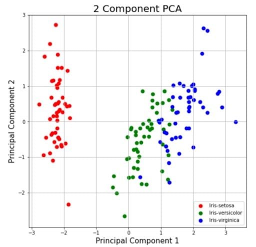

Explained Variance

The explained variance tells you how much information (variance) can be attributed to each of the principal components. This is important because while you can convert four-dimensional space to a two-dimensional space, you lose some of the variance (information) when you do this. By using the attribute explained_variance_ratio_, you can see that the first principal component contains 72.77 percent of the variance, and the second principal component contains 23.03 percent of the variance. Together, the two components contain 95.80 percent of the information.

pca.explained_variance_ratio_

PCA to Speed-Up Machine Learning Algorithms

While there are other ways to speed up machine learning algorithms, one less commonly known way is to use PCA. For this section, we aren’t using the Iris data set, as it only has 150 rows and four feature columns. The MNIST database of handwritten digits is more suitable, as it has 784 feature columns (784 dimensions), a training set of 60,000 examples and a test set of 10,000 examples.

Step 1: Download and Load the Data

You can also add a data_home parameter to fetch_mldata to change where you download the data.

from sklearn.datasets import fetch_openml
mnist = fetch_openml('mnist_784')

The images that you downloaded are contained in mnist.data and has a shape of (70000, 784) meaning there are 70,000 images with 784 dimensions (784 features).

The labels (the integers 0–9) are contained in mnist.target. The features are 784 dimensional (28 x 28 images), and the labels are numbers from 0–9.

Step 2: Split Data Into Training and Test Sets

The code below performs a train test split which puts 6/7th of the data into a training set and 1/7 of the data into a test set.

from sklearn.model_selection import train_test_split

# test_size: what proportion of original data is used for test set
train_img, test_img, train_lbl, test_lbl = train_test_split( mnist.data, mnist.target, test_size=1/7.0, random_state=0)

Step 3: Standardize the Data

The text in this paragraph is almost an exact copy of what was written earlier. PCA is affected by scale, so you need to scale the features in the data before applying PCA. You can transform the data onto unit scale (mean = 0 and variance = 1), which is a requirement for the optimal performance of many machine learning algorithms. StandardScaler helps standardize the data set’s features. You fit on the training set and transform on the training and test set.

from sklearn.preprocessing import StandardScaler
scaler = StandardScaler()

# Fit on training set only.
scaler.fit(train_img)

# Apply transform to both the training set and the test set.
train_img = scaler.transform(train_img)
test_img = scaler.transform(test_img)

Step 4: Import and Apply PCA

Notice the code below has .95 for the number of components parameter. It means that scikit-learn chooses the minimum number of principal components such that 95 percent of the variance is retained.

from sklearn.decomposition import PCA

# Make an instance of the Model
pca = PCA(.95)

Fit PCA on the training set. You are only fitting PCA on the training set.

pca.fit(train_img)

You can find out how many components PCA has after fitting the model using pca.n_components_. In this case, 95 percent of the variance amounts to 330 principal components.

Step 5: Apply the Mapping (transform) to the Training Set and the Test Set.

train_img = pca.transform(train_img)
test_img = pca.transform(test_img)

Step 6: Apply Logistic Regression to the Transformed Data

1. Import the model you want to use.

In sklearn, all machine learning models are implemented as Python classes.

from sklearn.linear_model import LogisticRegression

2. Make an instance of the model.

# all parameters not specified are set to their defaults
# default solver is incredibly slow which is why it was changed to 'lbfgs'
logisticRegr = LogisticRegression(solver = 'lbfgs')

3. Train the model on the data, storing the information learned from the data.

The model is learning the relationship between digits and labels.

logisticRegr.fit(train_img, train_lbl)

4. Predict the labels of new data (new images).

This part uses the information the model learned during the model training process. The code below predicts for one observation.

# Predict for One Observation (image)
logisticRegr.predict(test_img[0].reshape(1,-1))

The code below predicts for multiple observations at once.

# Predict for One Observation (image)
logisticRegr.predict(test_img[0:10])

Step 7: Measuring Model Performance

While accuracy is not always the best metric for machine learning algorithms (precision, recall, F1 score, ROC curve, etc., would be better), it is used here for simplicity.

logisticRegr.score(test_img, test_lbl)

Testing the Time to Fit Logistic Regression After PCA

The whole purpose of this section of the tutorial was to show that you can use PCA to speed up the fitting of machine learning algorithms. The table below shows how long it took to fit logistic regression on my MacBook after using PCA (retaining different amounts of variance each time).

More on Data ScienceUnderstanding Boxplots

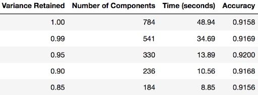
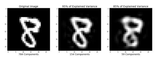
Image Reconstruction From Compressed Representation

Earlier sections of this tutorial demonstrated how to use PCA to compress high dimensional data to lower dimensional data. But PCA can also take the compressed representation of the data (lower dimensional data) and return it to an approximation of the original high dimensional data. If you are interested, you can use this code to reproduce the image below. 

I could’ve written so much more in this post about PCA, as it has many different uses. But I hope this helps you with whatever task you are working on.

Frequently Asked Questions