Data is skewed when the curve appears distorted to the left or right in a statistical distribution. In a normal distribution, the graph appears symmetrical, which means there are as many data values on the left side of the median as on the right side.
What Is Skewed Data?
Skewed data is data that creates an uneven curve distribution on a graph. We know data is skewed when the statistical distribution’s curve appears distorted to the left or right.
Let’s look at this height distribution graph as an example:
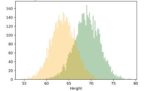
Here, you can see the green graph (males) has symmetry at about 69, and the yellow graph (females) has symmetry at about 64. So, it means that most of the males in this data set have a height near 69, and most females have a height near 64. Then there are a few males who have height near 75 and 63 and females who have height near to 68 and 58.
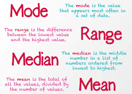
In the case of normal distribution, the mean, median and mode are close together. These three are all measures of the center of data. We can determine the skewness of the data by how these quantities relate to one another.
Right (or Positively) Skewed Data
A right-skewed distribution has a long tail that extends to the right or positive side of the x-axis, as you can see in the below plot.
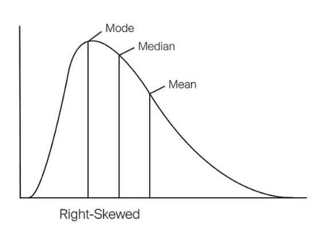
Here you can see the positions of all three data points on the plot. So, you see:
- The mean is greater than the mode.
- The median is greater than the mode.
- The mean is greater than the median.
While the mean and the median will always be greater than the mode in a right-skewed distribution, the mean may not always be greater than the median.
Let’s look at some real-world examples.
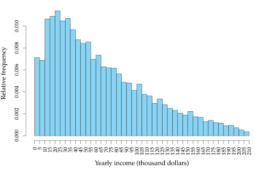
You can see this is right-skewed data with its tail in the positive side of the distribution. Here the distribution tells us that most people have incomes around $20,000 a year and the number of people with higher incomes exponentially decreases as we move to the right.
Now take a look at the following distribution from the 2002 General Social Survey. Respondents stated how many people older than 18 lived in their household.
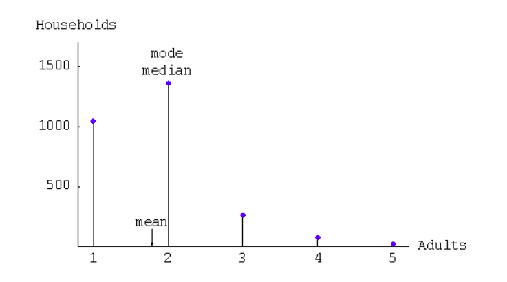
Here the distribution is skewed to the right. Although the mean is generally to the right of the median in a right-skewed distribution, that isn’t the case here.
Left (or Negatively) Skewed Data
A left-skewed distribution has a long tail that extends to the left (or negative) side of the x-axis, as you can see in the below plot.

Here you can see the positions of all three data points on the plot. So, you will find:
- The mean is greater than the mode.
- The median is greater than the mode.
- The mean is greater than the median.
While the mean and the median will always be greater than the mode in a right-skewed distribution, the mean may not always be greater than the median.
Let’s look at another real-world example.
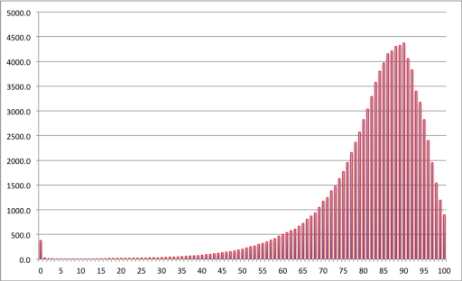
Here the distribution tells us most people die at an age of 90 (mode). Average life expectancy would be around 75 to 85 (mean). In the above distribution, you can see a small peak at the very beginning, which indicates there is a small percentage of the population who die during birth or in infancy. This population is acting as an outlier in our distribution.
My Data Is Skewed. So What?
Real-world distributions are usually skewed as we see in the above examples. But if there’s too much skewness in the data, then many statistical models don’t work effectively. Why is that?
In skewed data, extreme values in the tail can act as outliers, which may reduce the accuracy of certain models , and we know that outliers adversely affect a model’s performance, especially regression-based models. While there are statistical models that are robust enough to handle outliers like tree-based models, you’ll be limited in what other models you can try. So what do you do? You’ll need to transform the skewed data so that it becomes a Gaussian (or normal) distribution. Removing outliers and normalizing our data will allow us to experiment with more statistical models.
Log Transformation for Skewed Data
Log transformation is a data transformation method in which we apply logarithmic function to the data. It replaces each value x with log(x). A log transformation can help to fit a very skewed distribution into a Gaussian one. After log transformation, we can see patterns in our data much more easily. Here’s an example:
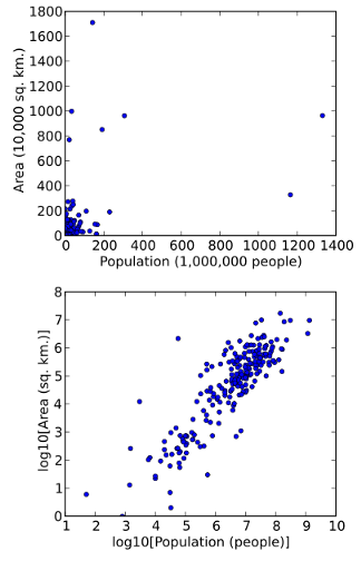
In the above figure, you can clearly see the patterns after applying log transformation. Before that, we had too many outliers present, which will negatively affect our model’s performance.
If we have skewed data, then it may, well, skew our results. A log transformation is often applied to positively skewed data, but it is only appropriate when all values are positive. Other transformations (square root, Box-Cox, Yeo-Johnson) may be better suited in different cases to discover patterns in the data and make it possible to draw insights from our statistical model.
Frequently Asked Questions
What is skewed data?
Skewed data is data that creates a skewed, asymmetrical statistical distribution, instead of following a Gaussian (normal) distribution. A skewed distribution on a graph has a curve distorted to the left or right of the graph’s center.
What problems does skewed data cause?
Skewed data indicates the existence of outliers in a data set, which can negatively affect statistical model performance and reduce model accuracy. Skewed data can also be difficult for some types of models to process, so this limits the amount of models available to use for analyzing the data set.
How do you ensure data isn't skewed?
To prevent skewed data, ensure that:
- Data sampling/collection is unbiased, representative of the larger population and performed as fairly as possible.
- Data is normalized (which can be done through transformations like logarithm, square root or square transformation).
- Outliers are understood and managed, which can include modifying or removing them from the data set if necessary.


