How to Use the Z-Table

A z-table shows the percentage or probability of values that fall below a given z-score in a standard normal distribution. A z-score shows how many standard deviations a certain value is from the mean in a distribution. Here’s how to use a z-table and interpret a z-score for your data.

What Is a Z-Score? 

A z-score, or a standard score, tells how many standard deviations a given value is from the mean value in a distribution. The standard deviation is a measure of how data points are dispersed in relation to the mean. Z-scores can be used with any distribution, but are often the most informative when applied to a symmetric, normal distribution (known as a bell curve or Gaussian distribution).
 

How to Calculate Z-Score 

The z-score formula is as follows:

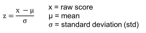
How to Interpret Z-Score

If a z-score is positive, the observed value is above the mean. If a z-score is negative, the value is below the mean. If a z-score is 0, the value is equal to the mean. For example, a z-score of 1.0 shows that the value is one standard deviation above the mean, while a z-score of -1.0 shows the value is one standard deviation below the mean.

What Is a Z-Table?

A z-table, or standard normal table, tells the percentage of values that are less than a given z-score. This percentage also represents the probability of a value falling within the area to the left of a z-score in a standard normal distribution. 

Z-tables can be positive or negative. A positive z-table is used when a z-score is positive, while a negative z-table is used when a z-score is negative. 

More on Data ScienceUnderstanding Boxplots

How to Use a Z-Table (With Example)

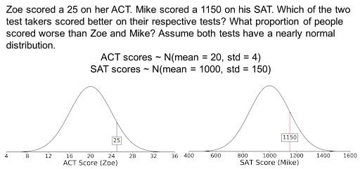
To explain how to use a z-table, let’s apply an example. Imagine a scenario where we compare the test results from two students, Zoe and Mike. Zoe took the ACT and scored a 25, while Mike took the SAT and scored 1150. Both of these scores are represented as normal distributions. Which of the test takers scored better? And what proportion of people scored worse than Zoe and Mike?

1. Calculate Z-Score 

To answer the above questions, we have to first use the z-score formula to calculate z-scores for Zoe and Mike.

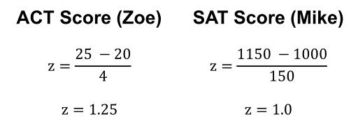
From these results, Zoe has a higher z-score than Mike. As such, Zoe performed better on her test.

Additionally, these test scores started as normal distributions, so finding their z-scores also converts them into standard normal distributions, where the mean is 0 and the standard deviation is 1 (N(mean = 0, std = 1)).

2. Use the Z-Score to Find Probability on a Z-Table 

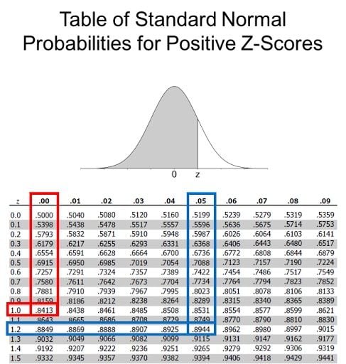
While we know that Zoe performed better than Mike because of her higher z-score, a z-table can tell you in what percentile each of the test takers are in. We will use a positive z-table since both Zoe’s and Mike’s z-scores are positive and greater than the mean value of 0. The following partial z-table — cut off to save space — can tell you the area underneath the curve to the left of our z-score. This is the percentage of students that scored less than Zoe or Mike.

3. Find Zoe’s Z-Score Probability

To use the z-table, start on the left side of the table and go down to 1.2. At the top of the table, go to 0.05. This corresponds to the value of 1.2 + .05 = 1.25. The value in the table is .8944 which is the probability. Roughly 89.44 percent of people scored worse than Zoe on the ACT.

4. Find Mike’s Z-Score Probability

Mike’s z-score was 1.0. To use the z-table, start on the left side of the table and go down to 1.0. Now at the top of the table, go to 0.00. This corresponds to the value of 1.0 + .00 = 1.00. The value in the table is .8413, which is the probability. Roughly 84.13 percent of people scored worse than Mike on the SAT.

How to Create a Z-Table 

This section will answer where the values in the z-table come from by going through the process of creating a z-score table. Please don’t worry if you don’t understand this section. It’s not important if you just want to know how to use a z-score table.
 

Finding the Probability Density Function

This is very similar to the 68–95–99.7 rule, but adapted for creating a z-table. Probability density functions (PDFs) are important to understand if you want to know where the values in a z-table come from. A PDF is used to specify the probability of the random variable falling within a particular range of values, as opposed to taking on any one value. This probability is given by the integral of this variable’s PDF over that range. That is, it’s given by the area under the density function but above the horizontal axis, and between the lowest and greatest values of the range.

This definition might not make much sense, so let’s clear it up by graphing the probability density function for a normal distribution. The equation below is the probability density function for a normal distribution

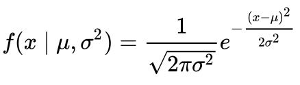
Let’s simplify it by assuming we have a mean (μ) of zero and a standard deviation (σ) of one (standard normal distribution).

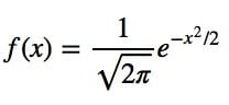
This can be graphed using any language, but I choose to graph it using Python.

# Import all libraries for this portion of the blog post
from scipy.integrate import quad
import numpy as np
import matplotlib.pyplot as plt
import pandas as pd
%matplotlib inline

x = np.linspace(-4, 4, num = 100)
constant = 1.0 / np.sqrt(2*np.pi)
pdf_normal_distribution = constant * np.exp((-x**2) / 2.0)
fig, ax = plt.subplots(figsize=(10, 5));
ax.plot(x, pdf_normal_distribution);
ax.set_ylim(0);
ax.set_title('Normal Distribution', size = 20);
ax.set_ylabel('Probability Density', size = 20);

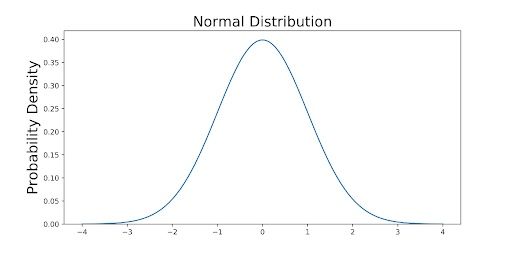
The graph above does not show you the probability of events but their probability density. To get the probability of an event within a given range, you need to integrate.

More on Data ScienceUnderstanding Train Test Split

Finding the Cumulative Distribution Function

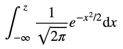
Recall that the standard normal table entries are the area under the standard normal curve to the left of z (between negative infinity and z).

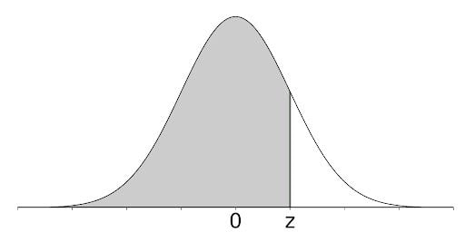
To find the area, you need to integrate. Integrating the PDF gives you the cumulative distribution function (CDF), which is a function that maps values to their percentile rank in a distribution. The values in the table are calculated using the cumulative distribution function of a standard normal distribution with a mean of zero and a standard deviation of one. This can be denoted with the equation below.

This is not an easy integral to calculate by hand, so I am going to use Python to calculate it. The code below calculates the probability for Zoe, who had a z-score of 1.25, and Mike, who had a z-score of 1.00.

def normalProbabilityDensity(x):
    constant = 1.0 / np.sqrt(2*np.pi)
    return(constant * np.exp((-x**2) / 2.0) )

zoe_percentile, _ = quad(normalProbabilityDensity, np.NINF, 1.25)
mike_percentile, _ = quad(normalProbabilityDensity, np.NINF, 1.00)
print('Zoe: ', zoe_percentile)
print('Mike: ', mike_percentile)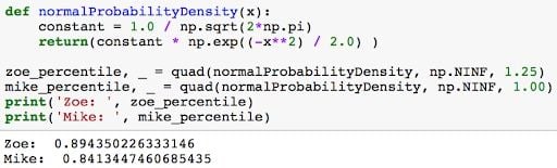

As the code below shows, these calculations can be done to create a z-table.

One important point to emphasize is that calculating this table from scratch when needed is inefficient, so we usually resort to using a standard normal table from a textbook or online source.

Why Are Z-Tables Important?

A z-table is able to present what percentage of data points in a distribution fall below a measured z-score. It can be used to compare two different z-scores from different distributions, or to shed light on other possible data probabilities based on hypothetical z-scores. Z-tables can be helpful for comparing data points and averages in cases like test scores, medical measurements or financial investments.

Frequently Asked Questions