")
The Markov decision process (MDP) is a mathematical framework used for modeling decision-making problems where the outcomes are partly random and partly controllable. It’s a framework that can address most reinforcement learning (RL) problems.
What Is the Markov Decision Process?
I’m going to describe the RL problem in a broad sense, and I’ll use real-life examples framed as RL tasks to help you better understand it.
Markov Decision Process Terminology
Before we can get into MDPs, we’ll need to review a few important terms that will be used throughout this article:
- Agent: A reinforcement learning agent is the entity which we are training to make correct decisions. For example, a robot that is being trained to move around a house without crashing.
- Environment: The environment is the surroundings with which the agent interacts. For example, the house where the robot moves. The agent cannot manipulate the environment; it can only control its own actions. In other words, the robot can’t control where a table is in the house, but it can walk around it.
- State: The state defines the current situation of the agent. This can be the exact position of the robot in the house, the alignment of its two legs or its current posture. It all depends on how you address the problem.
- Action: The choice that the agent makes at the current time step. For example, the robot can move its right or left leg, raise its arm, lift an object or turn right/left, etc. We know the set of actions (decisions) that the agent can perform in advance.
- Policy: A policy is the thought process behind picking an action. In practice, it’s a probability distribution assigned to the set of actions. Highly rewarding actions will have a high probability and vice versa. If an action has a low probability, it doesn’t mean it won’t be picked at all. It’s just less likely to be picked.
We’ll start with the basic idea of Markov Property and then continue to layer more complexity.
What Is the Markov Property?
Imagine that a robot sitting on a chair stood up and put its right foot forward. So, at the moment, it’s standing with its right foot forward. This is its current state.
Now, according to the Markov property, the current state of the robot depends only on its immediate previous state (or the previous timestep,) i.e. the state it was in when it stood up. And evidently, it doesn’t depend on its prior state– sitting on the chair. Similarly, its next state depends only on its current state.
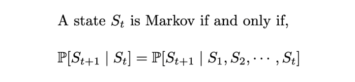
Formally, for a state S_t to be Markov, the probability of the next state S_(t+1) being s’ should only be dependent on the current state S_t = s_t, and not on the rest of the past states S₁ = s₁, S₂ = s₂, … .
Markov Process Explained

A Markov process is defined by (S, P) where S are the states, and P is the state-transition probability. It consists of a sequence of random states S₁, S₂, … where all the states obey the Markov property.
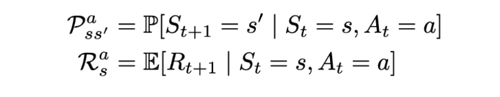
The state transition probability or P_ss’ is the probability of jumping to a state s’ from the current state s.
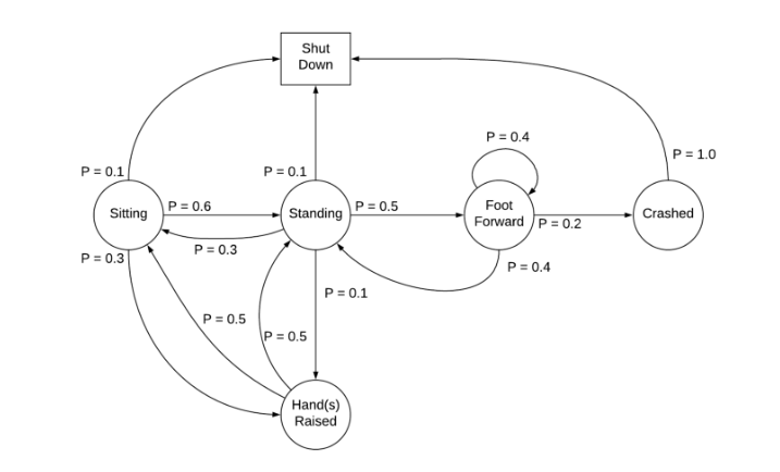
To understand the concept, consider the sample Markov chain above. Sitting, standing, crashed, etc., are the states, and their respective state transition probabilities are given.
Markov Reward Process (MRP)
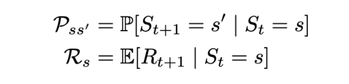
The Markov reward process (MRP) is defined by (S, P, R, γ), where S are the states, P is the state-transition probability, R_s is the reward, and γ is the discount factor, which will be covered in the coming sections.
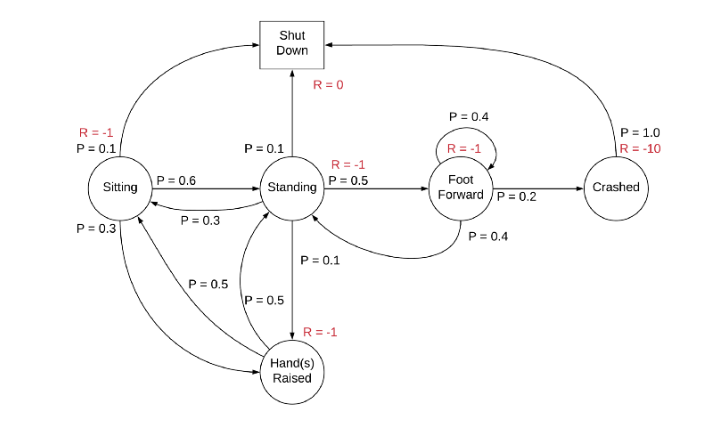
The state reward R_s is the expected reward over all the possible states that one can transition to from state s. This reward is received for being at the state S_t. By convention, it’s said that the reward is received after the agent leaves the state, and is hence regarded as R_(t+1).
For example:
Markov Decision Process (MDP)
A Markov decision process (MDP) is defined by (S, A, P, R, γ), where A is the set of actions. It is essentially MRP with actions. Introduction to actions elicits a notion of control over the Markov process. Previously, the state transition probability and the state rewards were more or less stochastic (random.) However, now the rewards and the next state also depend on what action the agent picks. Basically, the agent can now control its own fate (to some extent.)
Now, we will discuss how to use MDPs to address RL problems.
Return (G_t)
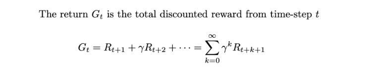
Rewards are temporary. Even after picking an action that gives a decent reward, we might be missing on a greater total reward in the long-run. This long-term total reward is the Return (G_t). However, in practice, we consider discounted Returns.
Discount (γ)
The variable γ ∈ [0, 1] in the figure is the discount factor. The intuition behind using a discount (γ) is that there is no certainty about the future rewards. While it is important to consider future rewards to increase the Return, it’s also equally important to limit the contribution of the future rewards to the Return (since you can’t be 100 percent certain of the future.)
And also because using a discount is mathematically convenient.
Policy (π)
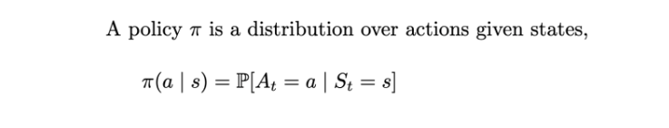
As mentioned earlier, a policy (π) defines the thought behind making a decision (picking an action). It defines the behavior of an RL agent.
Formally, a policy is a probability distribution over the set of actions a, given the current state s. It gives the probability of picking an action a at state s.
Value Functions
A value function is the long-term value of a state or an action. In other words, it’s the expected Return over a state or an action. This is something that we are actually interested in optimizing.
State Value Function for MRP

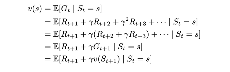
The state value function v(s) is the expected Return starting from state s.
Bellman Expectation Equation for Markov Reward Process (MRP)
The Bellman Equation gives a standard representation for value functions. It decomposes the value function into two components:
- The immediate reward
R_(t+1). - Discounted value of the future state
γ.v(S_(t+1)).
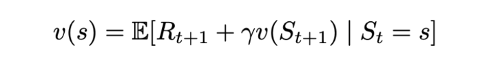
Let’s consider the following scenario (for simplicity, we’re going to consider MRPs only):
The agent can transition from the current state s to some state s’. Now, the state value function is basically the expected value of returns over all s’. Now, using the same definition, we can recursively substitute the return of the next state s’ with the value function of s’. This is exactly what the Bellman equation does:
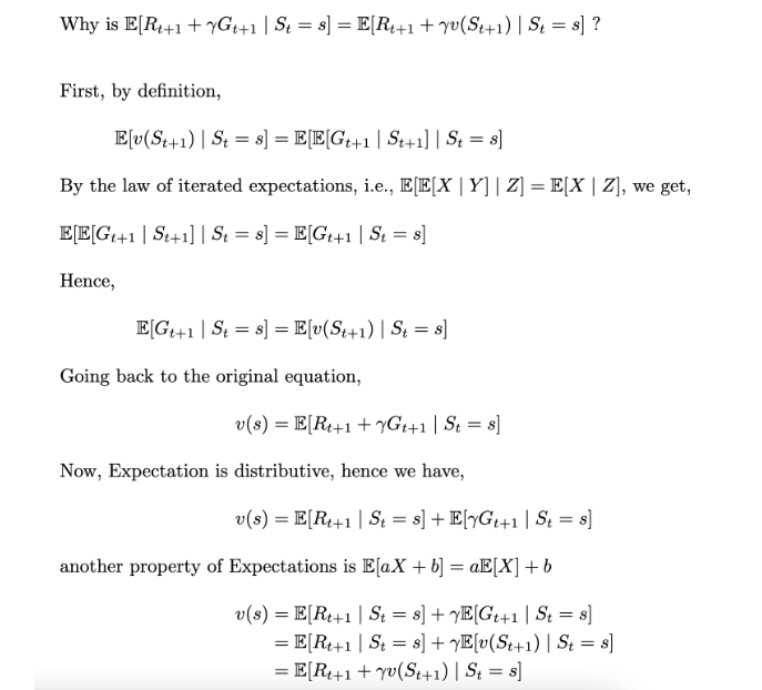
Now let’s solve this equation:
Solution for the value function. | Image: Rohan Jagtap
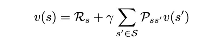
Since expectation is distributive, we can solve for both R_(t+1) and v(s’) separately. We have already seen that the expected value of R_(t+1) over S_t=s is the state reward R_s. And the expectation of v(s’) over all s’ is taken by the definition of expected value.
Another way of saying this would be — the state reward is the constant value that we are anyway going to receive for being at the state s. And the other term is the average state value over all s’.
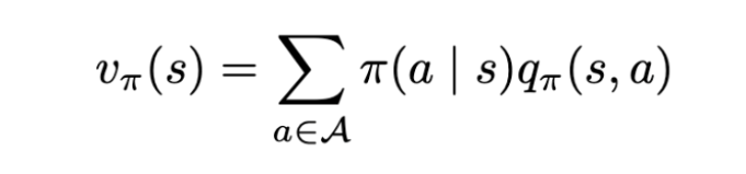
State Value Function for Markov Decision Process (MDP)
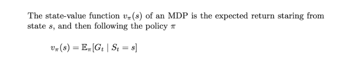
State value function for an MDP. | Image: Rohan Jagtap
This is similar to the value function for MRP, but there is a small difference that we’ll see shortly.
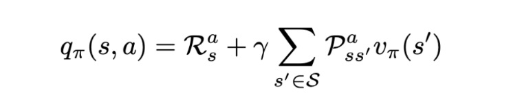
Action Value Function for Markov Decision Process (MDP)
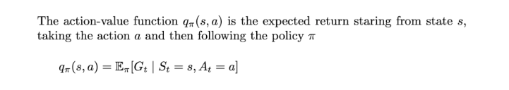
Action value function for an MDP. | Image: Rohan Jagtap
MDPs introduce control in MRPs by considering actions as the parameter for state transition. So, it is necessary to evaluate actions along with states. For this, we define action value functions that give us the expected Return over actions.
State value functions and action value functions are closely related. We’ll see how in the next section.
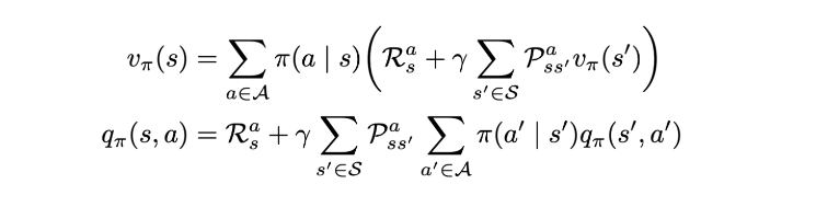
Bellman Expectation Equation (for MDP)
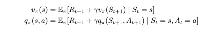
Bellman expectation equations for an MDP. | Image: Rohan Jagtap
Since we know the basics of the Bellman equation now, we can jump to the solution of this equation and see how this differs from the Bellman equation for MRPs:
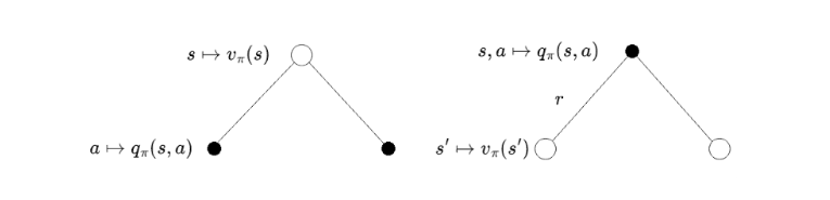
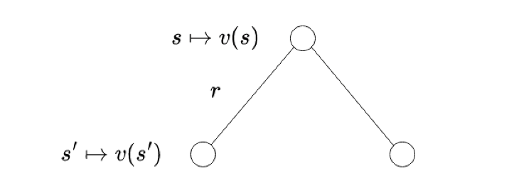
Intuition on Bellman equation. | Image: Rohan Jagtap
We represent the states using circles and actions using dots; both the diagrams above are a different level view of the same MDP. The left half of the image is the “state-centric” view and the right is the “action-centric” view.
Let’s first understand the figure:
- Circle to dot: The agent is in a state s; it picks an action a according to the policy. Say we’re training the agent to play chess. One time step is equivalent to one whole move (one white and one black move respectively.) In this part of the transition, the agent picks an action (makes a move.) The agent completely controls this part as it gets to pick the action part is completely controllable by the agent as it gets to pick the action.
- Dot to circle: The environment acts on the agent and sends it to a state based on the transition probability. Continuing the chess-playing agent example, this is the part of the transition where the opponent makes a move. After both moves, we call it a complete state transition. The agent can’t control this part as it can’t control how the environment acts, only its own behavior.
Now we treat these as two individual mini transitions:
Since we have a state to action transition, we take the expected action value over all the actions.
And this completely satisfies the Bellman equation as the same is done for the action value function:
Solution for the action value function. | Image: Rohan Jagtap
We can substitute this equation in the state value function to obtain the value in terms of recursive state value functions (and vice versa) similar to MRPs:
Markov Decision Process Optimal Value Functions
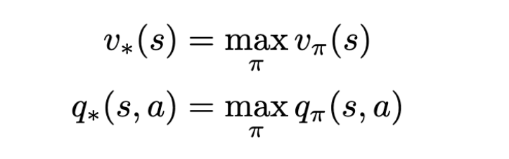
Imagine if we obtained the value for all the states/actions of an MDP for all possible patterns of actions that can be picked, then we could simply pick the policy with the highest value for the states and actions. The equations above represent this exact thing. If we obtain q∗(s, a), the problem is solved.
We can simply assign probability 1 for the action that has the max value for q∗ and 0 for the rest of the actions for all given states.
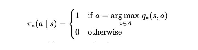
Optimal policy. | Image: Rohan Jagtap
Bellman Optimality Equation
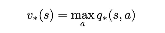
Bellman optimality equation for optimal state value function. | Image: Rohan Jagtap
Since we are anyway going to pick the action that yields the max q∗, we can assign this value as the optimal value function.
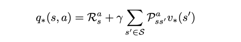
Bellman optimality equation for optimal action value function. | Image: Rohan Jagtap
Nothing much can change for this equation, as this is the part of the transition where the environment acts; the agent cannot control it. However, since we are following the optimal policy, the state value function will be the optimal one.
We can address most RL problems as MDPs like we did for the robot and the chess-playing agent. Just identify the set of states and actions.
In the previous section, I said, “Imagine if we obtained the value for all the states/actions of an MDP for all possible patterns of actions that can be picked….” However, this is practically infeasible. There can be millions of possible patterns of transitions, and we cannot evaluate all of them. However, we only discussed the formulation of any RL problem into an MDP, and the evaluation of the agent in the context of an MDP. We did not explore solving for the optimal values/policy.
There are many iterative solutions to obtain the optimal solution for the MDP. Some strategies to keep in mind as you move forward include:
- Value iteration.
- Policy iteration.
- SARSA.
- Q-learning.
Frequently Asked Questions
What is the Markov decision process?
A Markov decision process (MDP) is a stochastic (randomly-determined) mathematical tool based on the Markov property concept. It is used to model decision-making problems where outcomes are partially random and partially controllable, and to help make optimal decisions within a dynamic system. The Markov property expresses that in a random process, the probability of a future state occurring depends only on the current state, and doesn’t depend on any past or future states.
How do you know if a process is Markov?
A Markov process or Markov chain is a stochastic process of states that is memoryless, or where the probability of any future state (S_t+1) occurring is only dependent on its current state (S_t), and is independent of any past or future states.