What Is Descriptive Statistics?

In this article, I’ll help you understand the difference between descriptive statistics and inferential statistics. Then we’ll walk through some examples of descriptive statistics and how you can calculate them yourself.

What Is Statistics?

Statistics is the science of collecting data and analyzing them to infer proportions (sample) that are representative of the population. In other words, statistics is interpreting data in order to make predictions for the population.

There are two branches of statistics.

• Descriptive Statistics: Descriptive statistics is a statistical measure that describes data.
• Inferential Statistics: You practice inferential statistics when you use a random sample of data taken from a population to describe and make inferences about the population.

Descriptive Statistics vs. Inferential Statistics?

Descriptive statistics summarize data through certain numbers like mean, median, mode, etc. so as to make it easier to understand and interpret the data. Descriptive statistics don’t involve any generalization or inference beyond what is immediately available. This means that the descriptive statistics represent the available data (sample) and aren’t based on any theory of probability.

Commonly Used Measures

1. Measures of central tendency
2. Measures of dispersion (or variability)

What Are the Measures of Central Tendency?

A measure of central tendency is a one-number summary of the data that typically describes the center of the data. This one-number summary is of three types.

1. Mean
2. Median
3. Mode

1. What Is the Mean?

Mean is the ratio of the sum of all observations in the data to the total number of observations. This is also known as average. Thus, mean is a number around which the entire data set is spread.

More on StatisticsStatistical Tests: When to Use T-Test, Chi-Square and More

2. What Is the Median? 

Median is the point which divides the entire data into two equal halves. One half of the data is less than the median and the other half is greater than the median. Median is calculated by first arranging the data in either ascending or descending order.

• If the number of observations is odd, median is given by the middle observation in the sorted form.
• If the number of observations are even, median is given by the mean of the two middle observations in the sorted form.

An important point to note is that the order of the data (ascending or descending) does not affect the median.

3. What Is the Mode? 

Mode is the number that has the maximum frequency in the entire data set. In other words, mode is the number that appears the most often. A data can have one or more than one mode.

• If there is only one number that appears the most number of times, the data has one mode, and is called uni-modal.
• If there are two numbers that appear equally frequently, the data has two modes, and is called bi-modal.
• If there are more than two numbers that appear equally frequently, the data has more than two modes. We call that multi-modal.

How to Find the Mean, Median and Mode

Consider the following data points:

17, 16, 21, 18, 15, 17, 21, 19, 11, 23

We calculate the mean as:

To calculate the median, let’s arrange the data in ascending order:

11, 15, 16, 17, 17, 18, 19, 21, 21, 23

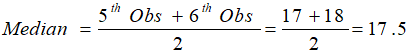
Since the number of observations is even (10), median is given by the average of the two middle observations (fifth and sixth here).

Mode is given by the number that occurs the most number of times. Here, 17 and 21 both occur twice. Hence, this is a bi-modal data set and the modes are 17 and 21.

A few things to note: 

1. Since median and mode don’t consider all the data points for calculations, median and mode are robust against outliers (i.e., these are not affected by outliers).
2. At the same time, mean shifts toward the outlier as it considers all the data points. This means if the outlier is big, mean overestimates the data, and if it is small, the data is underestimated.
3. If the distribution is symmetrical, mean = median = mode, or what we would call “normal distribution.”

More on DataHow to Find Outliers With IQR Using Python

What Are Measures of Dispersion?

Measures of dispersion describe the spread of the data around the central value (or the measures of central tendency).

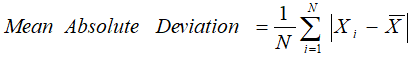
1. Absolute Deviation From Mean

The absolute deviation from the mean, also called mean absolute deviation (MAD), describes the variation in the data set. In a sense, it tells you the average absolute distance of each data point in the set. We calculate it as:  

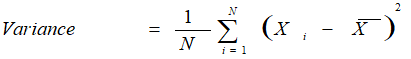
2. Variance

Variance measures how far data points spread out from the mean. A high variance indicates that data points are spread widely and a small variance indicates that the data points are closer to the data set’s mean. We calculate it as:

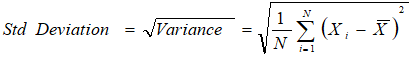
3. Standard Deviation

The square root of variance is called the standard deviation. We calculate it as:

Dive Into Probability Distributions4 Probability Distributions Every Data Scientist Needs to Know

4. Range

Range is the difference between the maximum value and the minimum value in the data set. It is given as:

5. Quartiles

Quartiles are the points in the data set that divides the data set into four equal parts. Q1, Q2 and Q3 are the first, second and third quartile of the data set.

• 25 percent of the data points lie below Q1 and 75 percent lie above it.
• 50 percent of the data points lie below Q2 and 50 percent lie above it. Q2 is nothing but median.
• 75 percent of the data points lie below Q3 and 25 percent lie above it.

More on QuartilesCalculating Quartiles: A Step-by-Step Explaination

6. Skewness

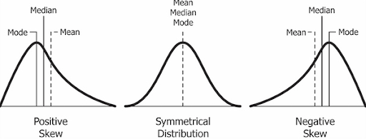
The measure of asymmetry in a probability distribution is defined by skewness. Skewness can either be positive, negative or undefined. We’ll focus on positive and negative skew.

• Positive Skew: This is the case when the tail on the right side of the curve is bigger than that on the left side. For these distributions, the mean is greater than the mode.
• Negative Skew: This is the case when the tail on the left side of the curve is bigger than that on the right side. For these distributions, mean is smaller than the mode.

The most commonly used method of calculating skewness is:

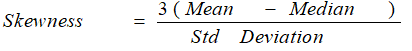
If the skewness is zero, the distribution is symmetrical. If it is negative, the distribution is negatively skewed and if it is positive, it is positively skewed.

7. Kurtosis

Kurtosis describes whether the data is light tailed (lack of outliers) or heavy tailed (outliers present) when compared to a normal distribution. There are three kinds of kurtosis:

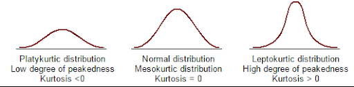
• Mesokurtic: This is the case when the kurtosis is zero, similar to normal distributions.
• Leptokurtic: This is when the tail of the distribution is heavy (outlier present) and kurtosis is higher than that of the normal distribution.
• Platykurtic: This is when the tail of the distribution is light (no outlier) and kurtosis is lesser than that of the normal distribution.