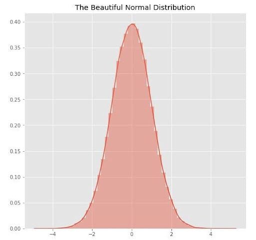
Box-Cox transformation is a statistical technique that transforms your target variable so that your data closely resembles a normal distribution.
In many statistical techniques, we assume that the errors are normally distributed. This assumption allows us to construct confidence intervals and conduct hypothesis tests. By transforming your target variable, we can hopefully normalize our errors, if they are not already normal.

Additionally, transforming our variables can improve the predictive power of our models because transformations can present white noise as a more normal distribution, limiting the impact of noise on the model’s performance.
What Is Box-Cox Transformation and Target Variable?
Box-Cox transformation is a statistical technique that involves transforming your target variable so that your data follows a normal distribution. A target variable is the variable in your analytical model that you are trying to estimate. Box-Cox transformation helps to improve the predictive power of your analytical model when dealing with white noise.
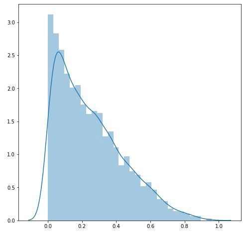
Suppose we had a beta distribution, where alpha equals one and beta equals three. If we plot this distribution, then it might look something like below:
plt.figure(figsize = (8, 8))
data = np.random.beta(1, 3, 5000)
sns.distplot(data)
plt.show()
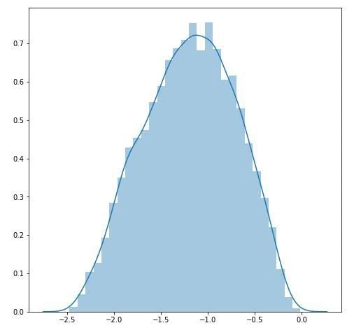
We can use the Box-Cox transformation to turn the above into as close to a normal distribution as the Box-Cox transformation permits.
tdata = boxcox(data)[0]
plt.figure(figsize = (8, 8))
sns.distplot(tdata)
plt.show()
And now our data looks more like a normal distribution.
What Is a Target Variable?
A target variable is the variable that you are trying to estimate. What’s nice about the linear regression model is that your target variable can take on virtually any form: continuous, ordinal, binary and more.
However, different forms of target variables will yield different interpretations of your slope parameters. For example, if your target variable is binary — that is, it takes on a value of either one or zero — then the slope parameters of your regression model represent the way a one-unit increase in your independent variables changes the probability that your target variable will equal one.
What Is the Box-Cox Transformation Equation?
If w is our transformed variable and “y” is our target variable, then the Box-Cox transformation equation looks like this:

In this equation, “t” is the time period and lambda is the parameter that we choose. You can also perform the Box-Cox transformation on non-time series data.
Notice what happens when lambda equals one. In that case, the transformation has little impact. If the optimal value for lambda is one, then the data is already normally distributed, and the Box-Cox transformation is unnecessary.
How Do You Choose Lambda?
We choose the value of lambda that provides the best approximation for the normal distribution of our response variable.
SciPy has a boxcox function that will choose the optimal value of lambda for us.
scipy.stats.boxcox()
Simply pass a 1-D array into the function and it will return the Box-Cox transformed array and the optimal value for lambda. You can also specify a number, alpha, which calculates the confidence interval for that value. For example, alpha = 0.05 gives the 95 percent confidence interval.
If llf is the log-likelihood function, then the confidence interval for lambda can be written as:

In this equation, “X²” is the chi-squared distribution. It may also be unnecessary to use the Box-Cox transformation if the confidence interval for lambda includes one since the data is already close to being normally distributed.
Next, fit your model to the Box-Cox transformed data. You must revert your data to its original scale when you are ready to make predictions.
For example, your model might predict that the Box-Cox transformed value, given other features, is 1.5. You need to take that 1.5 and revert it to its original scale — the scale of your target variable.
Thankfully, SciPy also has a function for this.
scipy.special.inv_boxcox(y, lambda)Enter the data you want to transform, “y,” and the lambda with which you had transformed your data.
Limits of Box-Cox Transformation
If interpretation is your goal, then the Box-Cox transformation may be a poor choice. If lambda is a non-zero number, then the transformed target variable may be more difficult to interpret than if we simply applied a log transform.
A second issue is that the Box-Cox transformation usually gives the median of the forecast distribution when we revert the transformed data to its original scale. Occasionally, we want the mean, not the median, and there are other ways to do that.
Now you know about the Box-Cox transformation, its implementation in Python, as well as its limitations.
Frequently Asked Questions
What is the purpose of the Box-Cox transformation?
The Box-Cox transformation is intended to adjust a non-normal variable so that it more closely follows a normal distribution. This can greatly improve the performance of a statistical model, even when dealing with white noise.
Why is normality important in statistical modeling?
Various types of statistical tests and techniques assume that data is normally distributed. If a data set isn’t normally distributed, this can impact the accuracy of these statistical models.
Can the Box-Cox transformation be applied to any data set?
No, the Box-Cox transformation assumes that all data points are positive and continuous, meaning that all values must be above zero. If this is not the case, the data must be adjusted so that all data points are positive before applying the Cox-Box transformation.


