Logistic regression is a classic machine learning algorithm used for classifying tasks. Mathematically, the logistic regression algorithm can be derived as a special case of the classical neural network algorithm used in deep learning. That is, if we shrink down a classical neural network to just one neuron, we get the logistic regression algorithm.
4 Steps to Create Neural Network Logistic Regression Code
- Create the Sigmoid function.
- Build the class.
- Fit the data.
- Create a predict method.
In the following post, we’ll explore how we can view the logistic regression algorithm as a one neuron neural network, write code for the same, and finally, ensure that our code is optimized (or vectorized).
Understanding the Mathematics Behind a Logistic Regression Algorithm as a Neural Network
There are three parts to the mathematics behind a logistic regression algorithm. Here's how it works:
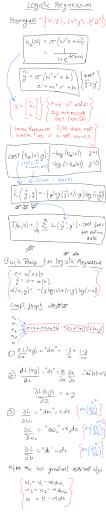
Logistic Regression Algorithm Mathematics
We start by writing down the algorithm’s mathematics and defining a linear function with random weights equal to the number of features provided, and a bias to fit onto our data. This can be thought of as fitting a straight line on our data if the number of features (x) is one.
We then pass the output of this linear function into a non-linear function, here a sigmoid function, to squish the output between 0 and 1, which will give us our non-linear logistic regression curve.
The next thing we need is a loss function to calculate how well our algorithm is doing, and we choose the standard one — binary cross-entropy loss or log loss — which is then summed up over the data to calculate the cost function.
The last thing we need is backpropagation, where we calculate the partial derivatives (for gradient descent) in the opposite direction of the conventional flow.
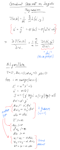
Calculating Gradient descent
Our next step would be to fit our data by running the classic gradient descent algorithm. For this, we write a pseudocode for the backpropagation step shown above to compute all the required derivatives. Then, we use these derivatives and the learning rate to adjust our parameters over several epochs, or until our cost function converges.
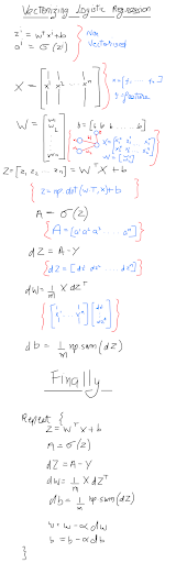
Vectorizing Logistic Regression
Our final step would be to make our algorithm efficient by getting rid of the for loops. We do so by treating everything as matrices so that we can perform matrix operations on the whole dataset in a single go using numpy .
Neural Networks Logistic Regression Sample Code in Python
Finally, we’ll implement the algorithm explained above step by step in Python.
1. Create the Sigmoid Function
Starting with the easiest bit, let us create the sigmoid function (a class method).
def sigmoid(self, z):
    """
    Returns sigmoid value.
    """
    return 1 / (1 + np.exp(-z))
2. Build the Class
Next, let us build a class that accepts features, labels, a debug flag (for printing logs), and alpha (for the gradient descent algorithm) as arguments. The class will include methods for our activation function (sigmoid), fitting data and predicting results. All the functions will work on arrays; hence, most of the code is vectorized to efficiently perform operations on the entire array in one pass. The docstrings of each method explains what part of the pipeline it carries out.
class LogisticRegression:
    """
    Logistic Regression using neural network.
    Parameters
    ==========
    X : np.ndarray
        Features to train a model. Should be of the form -
        [
            [feature1dataset1, feature1dataset2, .... feature1datasetn],
            [feature2dataset1, feature2dataset2, .... feature2datasetn],
            [feature3dataset1, feature3dataset2, .... feature3datasetn],
        ]
    Y : np.ndarray
        Labels to train the model. Should be of the form -
        [
            label1,
            label2,
            label3
        ]
    alpha : numerical (optional)
        The learning rate to be used.
    debug : bool
        To print debug statements.
    """

    def __init__(self, X, Y, alpha=0.05, debug=False):
        self.X = X
        self.Y = Y
        self.debug = debug
        self.alpha = alpha
        self.m = len(self.X)
3. Fit the Data
Now comes the main part of the code, the fit method. We start by initializing the cost function (J) and the previously seen cost function (J_last).
Next, we create an empty array for W (weights), dW (a derivative of the loss function w.r.t. weights) and create an infinite loop that breaks when the cost function starts converging, when the difference in two consecutive values of the cost function is less than 1e-5.
The loop performs all the mathematics explained above and finds the appropriate weights for our data (by running gradient descent).
def fit(self):
    """
    Maths involved -
    z = w.T * x + b
    y_predicted = a = sigmoid(z)
    dw += (1 / m) * x * dz
    db += dz
    Gradient descent -
    w = w - α * dw
    b = b - α * db
    """
    self.J = 0
    self.J_last = 1
    dW = np.zeros(shape=(self.m, 1))
    self.b = 0
    self.W = np.zeros(shape=(self.m, 1))

    while True:
        Z = np.dot(self.W.T, self.X) + self.b
        A = np.array([self.sigmoid(x) for x in Z])
        dZ = A - self.Y
        dW = (1 / self.m) * (np.dot(self.X, dZ.T))
        db = (1 / self.m) * np.sum(dZ)

        self.J = -np.sum(
            np.multiply(self.Y.T, np.array([np.log(x) for x in A.T]))
            + np.multiply(1 - self.Y.T, np.array([np.log(1 - x) for x in A.T]))
        )

        self.W = self.W - self.alpha * dW
        self.b = self.b - self.alpha * db

        if self.debug:
            print(self.J)

        if abs(self.J - self.J_last) < 1e-5:
            break
        else:
            self.J_last = self.J
4. Create a Predict Method
Finally, now we can create a predict method to utilize the calculated weights for predicting outputs. For this, we take in a list of features and iterate through each data to assign it either 1 or 0 using our good, old sigmoid function.
def predict(self, x):
    """
    Predicts the y values based on the training data.
    """
    prediction = []
    for single_data in x:
      prediction.append(
          1 if self.sigmoid(np.dot(single_data, self.W) + self.b) > 0.5 else 0
      )

    return prediction
The Complete Code
The complete class with some predictions:
import numpy as np
from sklearn.datasets import load_digits


class LogisticRegression:
    """
    Logistic Regression using neural network.
    Parameters
    ==========
    X : np.ndarray
        Features to train a model. Should be of the form -
        [
            [feature1dataset1, feature1dataset2, .... feature1datasetn],
            [feature2dataset1, feature2dataset2, .... feature2datasetn],
            [feature3dataset1, feature3dataset2, .... feature3datasetn],
        ]
    Y : np.ndarray
        Labels to train the model. Should be of the form -
        [
            label1,
            label2,
            label3
        ]
    alpha : numerical (optional)
        The learning rate to be used.
    debug : bool
        To print debug statements.
    """

    def __init__(self, X, Y, alpha=0.05, debug=False):
        self.X = X
        self.Y = Y
        self.debug = debug
        self.alpha = alpha
        self.m = len(self.X)

    def fit(self):
        """
        Maths involved -
        z = w.T * x + b
        y_predicted = a = sigmoid(z)
        dw += (1 / m) * x * dz
        db += dz
        Gradient descent -
        w = w - α * dw
        b = b - α * db
        """
        self.J = 0
        self.J_last = 1
        dW = np.zeros(shape=(self.m, 1))
        self.b = 0
        self.W = np.zeros(shape=(self.m, 1))

        while True:
            Z = np.dot(self.W.T, self.X) + self.b
            A = np.array([self.sigmoid(x) for x in Z])
            dZ = A - self.Y
            dW = (1 / self.m) * (np.dot(self.X, dZ.T))
            db = (1 / self.m) * np.sum(dZ)

            self.J = -np.sum(
                np.multiply(self.Y.T, np.array([np.log(x) for x in A.T]))
                + np.multiply(1 - self.Y.T, np.array([np.log(1 - x) for x in A.T]))
            )

            self.W = self.W - self.alpha * dW
            self.b = self.b - self.alpha * db

            if self.debug:
                print(self.J)

            if abs(self.J - self.J_last) < 1e-5:
                break
            else:
                self.J_last = self.J

    def sigmoid(self, z):
        """
        Returns sigmoid value.
        """
        return 1 / (1 + np.exp(-z))

    def predict(self, x):
        """
        Predicts the y values based on the training data.
        """
        prediction = []
        for single_data in x:
            prediction.append(
                1 if self.sigmoid(np.dot(single_data, self.W) + self.b) > 0.5 else 0
            )

        return prediction


if __name__ == "__main__":
    digits = load_digits()

    # preprocessing
    x_train = digits.data[:-797].T

    y = np.zeros(shape=(len(digits.target), 1))
    for i in range(len(digits.target)):
        if digits.target[i] == 2:
            y[i] = 1
        else:
            y[i] = 0

    y_train = y[:-797]

    model = LogisticRegression(x_train, y_train.T, alpha=0.01, debug=True)
    model.fit()
    pre = model.predict(np.array(digits.data[-797:])) - y[-797:].flatten()
    print(np.where(pre != 0))
Frequently Asked Questions
What is logistic regression?
Logistic regression is a classic machine learning algorithm used for classifying tasks. It can be derived as a special case of the classical neural network algorithm.
How do you implement logistic regression code in Python?
- Create the Sigmoid function.
- Build the class.
- Fit the data.
- Create a predict method.
What is an example of neural network logistic regression sample code in Python?
The following is sample code for a neural network logistic regression algorithm.
import numpy as np
from sklearn.datasets import load_digits


class LogisticRegression:
    """
    Logistic Regression using neural network.
    Parameters
    ==========
    X : np.ndarray
        Features to train a model. Should be of the form -
        [
            [feature1dataset1, feature1dataset2, .... feature1datasetn],
            [feature2dataset1, feature2dataset2, .... feature2datasetn],
            [feature3dataset1, feature3dataset2, .... feature3datasetn],
        ]
    Y : np.ndarray
        Labels to train the model. Should be of the form -
        [
            label1,
            label2,
            label3
        ]
    alpha : numerical (optional)
        The learning rate to be used.
    debug : bool
        To print debug statements.
    """

    def __init__(self, X, Y, alpha=0.05, debug=False):
        self.X = X
        self.Y = Y
        self.debug = debug
        self.alpha = alpha
        self.m = len(self.X)

    def fit(self):
        """
        Maths involved -
        z = w.T * x + b
        y_predicted = a = sigmoid(z)
        dw += (1 / m) * x * dz
        db += dz
        Gradient descent -
        w = w - α * dw
        b = b - α * db
        """
        self.J = 0
        self.J_last = 1
        dW = np.zeros(shape=(self.m, 1))
        self.b = 0
        self.W = np.zeros(shape=(self.m, 1))

        while True:
            Z = np.dot(self.W.T, self.X) + self.b
            A = np.array([self.sigmoid(x) for x in Z])
            dZ = A - self.Y
            dW = (1 / self.m) * (np.dot(self.X, dZ.T))
            db = (1 / self.m) * np.sum(dZ)

            self.J = -np.sum(
                np.multiply(self.Y.T, np.array([np.log(x) for x in A.T]))
                + np.multiply(1 - self.Y.T, np.array([np.log(1 - x) for x in A.T]))
            )

            self.W = self.W - self.alpha * dW
            self.b = self.b - self.alpha * db

            if self.debug:
                print(self.J)

            if abs(self.J - self.J_last) < 1e-5:
                break
            else:
                self.J_last = self.J

    def sigmoid(self, z):
        """
        Returns sigmoid value.
        """
        return 1 / (1 + np.exp(-z))

    def predict(self, x):
        """
        Predicts the y values based on the training data.
        """
        prediction = []
        for single_data in x:
            prediction.append(
                1 if self.sigmoid(np.dot(single_data, self.W) + self.b) > 0.5 else 0
            )

        return prediction


if __name__ == "__main__":
    digits = load_digits()

    # preprocessing
    x_train = digits.data[:-797].T

    y = np.zeros(shape=(len(digits.target), 1))
    for i in range(len(digits.target)):
        if digits.target[i] == 2:
            y[i] = 1
        else:
            y[i] = 0

    y_train = y[:-797]

    model = LogisticRegression(x_train, y_train.T, alpha=0.01, debug=True)
    model.fit()
    pre = model.predict(np.array(digits.data[-797:])) - y[-797:].flatten()
    print(np.where(pre != 0))