Linear regression is a fundamental method in statistics and machine learning. It allows a data scientist to model the relationship between an outcome variable and predictor variables. From this, the model can make predictions about test data. Yet, as the name suggests, linear regression assumes that outcome and predictor variables have a linear relationship, which isn’t the case in all data sets.
Luckily, polynomial regression allows for the accurate modeling of non-linear relationships. In this article, I’ll explain what polynomial regression models are and how to fit and evaluate them.
What Is Polynomial Regression?
Polynomial regression is an extension of a standard linear regression model. Polynomial regression models the non-linear relationship between a predictor and an outcome variable using the Nth-degree polynomial of the predictor.
Polynomial Regression Equation
To understand the structure of a polynomial regression model, let’s consider an example where one is appropriate.
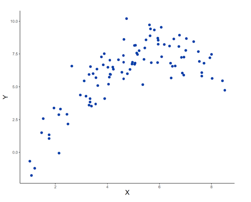
In the simulated data above, the predictor variable on the x-axis is not linearly related to the outcome variable on the y-axis. Instead, the relationship between these variables is better described by a curve. If we fit a linear regression model to these data, the model equation would be as follows:
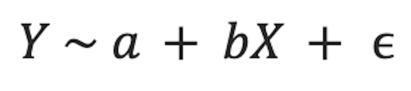
where a is the intercept (the value at which the regression line cuts through the y-axis), b is the coefficient, and ϵ is an error term.
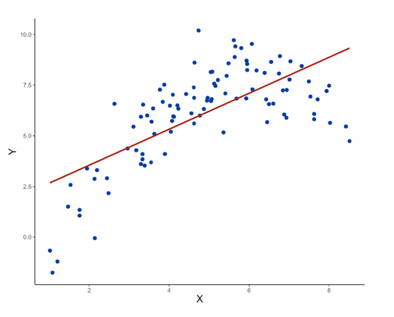
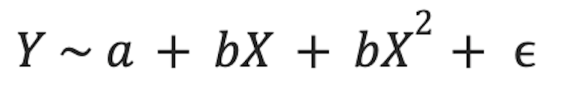
As seen in the plot above, this straight-line equation doesn’t do a good job of capturing the non-linear relationship in the data. To address this, we can fit a polynomial regression model. This model is an extension of the previous one, but X is now added again as a second-degree polynomial. The equation for this model is
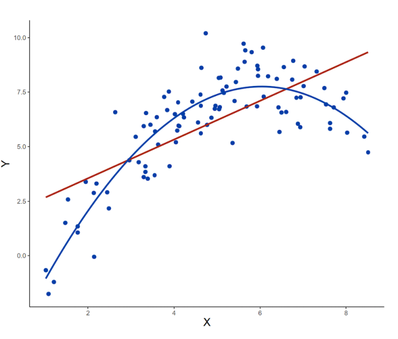
It’s clear from a quick visual inspection that the polynomial model gives a closer fit to the curved data. This will lead to more accurate predictions of new values in test data.
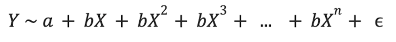
If necessary, more polynomial components can be added to the regression equation to fit more complex non-linear relationships. These would make the regression equation take this form:
So, how can you fit a polynomial regression model, and how can you tell when it includes too many components?
How to Fit a Polynomial Regression Model
The standard method for fitting both linear and polynomial regression in R is the method of least squares. This involves minimizing the sum of the squared residuals in the model by adjusting the values of the intercept and coefficients. The lm function in R minimizes the sum of squares for us, so all we need to do is specify the model. We can start by fitting a simple linear regression model to our example data.
model1 <- lm(Y ~ X, data = example_data)
summary(model1)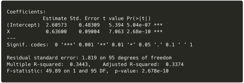
The summary above shows us the adjusted R² value for the model, which is a measure of how well the model predicts our outcome. An R2 equal to zero means the model accounts for none of the variance in the outcome, whereas one would mean it accounts for all the variance. In this case, R2 equals 0.34, meaning that our regression model accounts for 34 percent of the variance in the outcome variable. This is OK, but given the shape of the data, it makes sense to try adding a polynomial term to the model.
It’s easy to specify a polynomial regression model in R. It’s the same as linear regression, but we use the poly function to state that we want to add a polynomial term to our predictor and the power in the term itself. In this example, we fit a model with a quadratic component — a second-degree polynomial.
model2 <- lm(Y ~ poly(X, 2), data = example_data)
summary(model2)
It’s clear from the model summary that the polynomial term has improved the fit of the regression. R² now equals 0.81, a large increase from the previous model. But, just like in multiple regression, adding more terms to a model will always improve the fit. It is therefore essential to test whether this improvement in model fit is substantial enough to be considered meaningful.
How to Evaluate a Polynomial Regression Model
To justify adding polynomial components to a regression model, it’s important to test whether each one significantly improves the model fit. To do this, we can compare the fit of both models using an analysis of variance (ANOVA).
anova(model1, model2)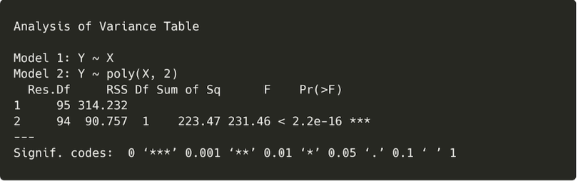
The results of this ANOVA are significant. The p-value (shown under “Pr(>F)” in the output) is very small and well below 0.05, the typical threshold for statistical significance. This means that adding the polynomial term helped the second regression model give a substantially better fit to the data than the first.
We can keep expanding the model and testing whether successive terms improve the fit. When more advanced terms no longer significantly improve the model fit, we have our final model specification. Testing whether a cubic polynomial term (a third-degree polynomial) to the model demonstrates this outcome.
model3 <- lm(Y ~ poly(X, 3), data = example_data)
summary(model3)
anova(model2, model3)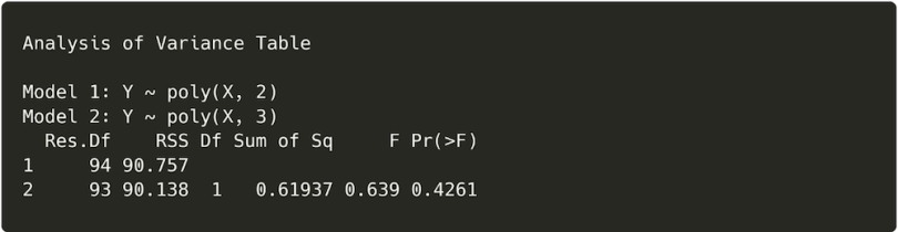
Here, the ANOVA is no longer significant, meaning that the cubic component didn’t substantially improve the model fit. This means we can leave out the cubic component and choose model2 as our final model.
How to Fit and Evaluate Polynomial Regression Models With Bayesian Methods
To fit polynomial regression models using Bayesian methods, you’ll need the BayesFactor R package. This includes the lmBF function; the Bayesian equivalent of the lm function.
To specify a polynomial regression equation in lmBF, we can’t use the poly function like in the lm example. This is because an error occurs if we try to use poly inside lmBF. To get around this, we can create a new column in our data that contains a polynomial term and then insert that as a coefficient in the model as shown below.
library(BayesFactor)
example_data$X_poly2 <- poly(example_data$X, 2)[,"2"]
BF_poly2 <- lmBF(Y ~ X + X_poly2, data = as.data.frame(example_data))
BF_poly2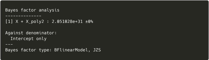
This outputs a Bayes factor for the regression, which is a measure of the evidence for our regression model versus a model with no coefficients. This gives us an idea of whether or not all of the predictors do a good job of explaining variance in our outcome. Bayes factors above three are often interpreted as being sufficient evidence in a model’s favor. Ours in this case is much greater, meaning the model is 2.05 × 1031 times more likely than one with no predictors.
This Bayes factor doesn’t tell us how useful each individual predictor is at improving the model fit, however. For this, we’ll need to compare models. To test whether the quadratic polynomial component improves our model fit, we can fit a simpler linear model with lmBF. Then, we divide the Bayes factor of our polynomial model by the Bayes factor of the simpler model. The resulting Bayes factor can be interpreted as the ratio of evidence for the complex model versus the simpler one.
BF_simple <- lmBF(Y ~ X, data = as.data.frame(example_data))
BF_poly2 / BF_simple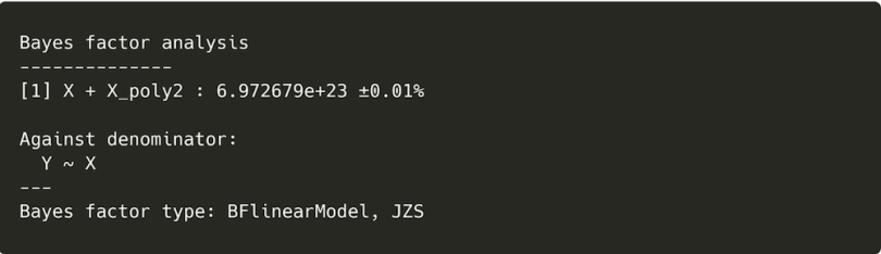
This value is once again very large, indicating sufficient evidence that the polynomial component is reliably improving the model fit. Based on this, we’d choose the polynomial regression model over the simple linear regression model.
Strengths and Limitations of Polynomial Regression
While polynomial regression is useful, it should be used with caution. Although it’s possible to add lots of polynomial components to a model to improve its fit, this increases the risk of overfitting. Overfitting is when a model fits the training data set very closely but is not generalizable enough to make accurate predictions about test data.
In an extreme case, a model with many polynomial terms could fit a training data set nearly perfectly, drawing a wavy line through all the data points. A model like this would be unable to generalize to new data, however, and would give all sorts of inaccurate predictions because it picked up so much of the random variation in the training data. This inaccuracy could lead you to make misinformed conclusions from your model, so you must avoid it.
To avoid overfitting, it’s important to test that each polynomial component in a regression model makes a meaningful difference to the model fit. By doing this, your model will include only the essential components needed to predict the outcome of interest. Because it avoids unnecessary complexity, it will therefore return more accurate predictions about test data.
Polynomial regression is also more sensitive to outliers than linear regression. In linear regression, outliers don’t usually have substantial effects on the model coefficients unless the outlying values themselves are very large. In contrast, one or two outlying values might change the whole specification of a polynomial regression model. Again, this can lead polynomial regression models to make inaccurate predictions.
With these limitations in mind, polynomial regression is a useful method for modelling non-linear relationships between predictor and outcome variables. As demonstrated, polynomial regression models give more accurate predictions about test data than linear regression in these cases. When used carefully, it is a powerful and versatile tool that belongs in any data scientist’s skill set.