The dot product of a matrix describes calculating the dot product of the corresponding rows and columns between two matrices.
A dot product is the sum of the products of corresponding elements between two vectors. Calculating the dot product of two matrices is done to perform matrix multiplication and create a new matrix from them, known as the matrix product.
What Is the Dot Product of a Matrix?
A dot product of a matrix is a basic linear algebra computation used in deep learning models to complete operations with larger amounts of data more efficiently. It’s the result of multiplying two matrices that have matching rows and columns, such as a 3x2 matrix and a 2x3 matrix. It can also be calculated in NumPy using the np.dot operation.
Machine learning and deep learning models often rely on large data sets for accuracy. As data volume increases, scalar operations can slow processing, making vectorized operations such as the dot product essential for efficient computation.
Linear algebra is one of the most important topics in the data science domain. In this post, we will cover dot product and matrix multiplication — two basic, yet important linear algebra operations that serve as the building blocks of complex machine learning and deep learning models.
How to Calculate the Dot Product of Two Vectors
The dot product of two vectors is the sum of the products of elements with regards to position. The first element of the first vector is multiplied by the first element of the second vector, and so on. The sum of these products is the dot product, which can be calculated with the np.dot() function from NumPy in Python.
Let’s first create two simple vectors in the form of NumPy arrays and calculate the dot product.

The dot product of these two vectors is the sum of the products of elements at each position. In this case, the dot product is (1*2)+(2*4)+(3*6).
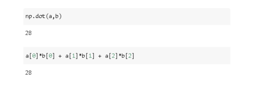
Since we multiply elements at the same positions, the two vectors must have the same length in order to have a dot product.
How to Calculate the Dot Product of Two Matrices
In data science, we mostly deal with matrices. A matrix is a bunch of row and column vectors combined in a structured way. Thus, the multiplication of matrices involves many dot product operations of vectors.
The multiplication of two matrices involves dot products between the rows of the first matrix and the columns of the second matrix.
It will be more clear when we go over some examples. Let’s first create two, 2x2 matrices with NumPy.

Two, 2x2 Num{y arrays. | Image: Soner Yildirim

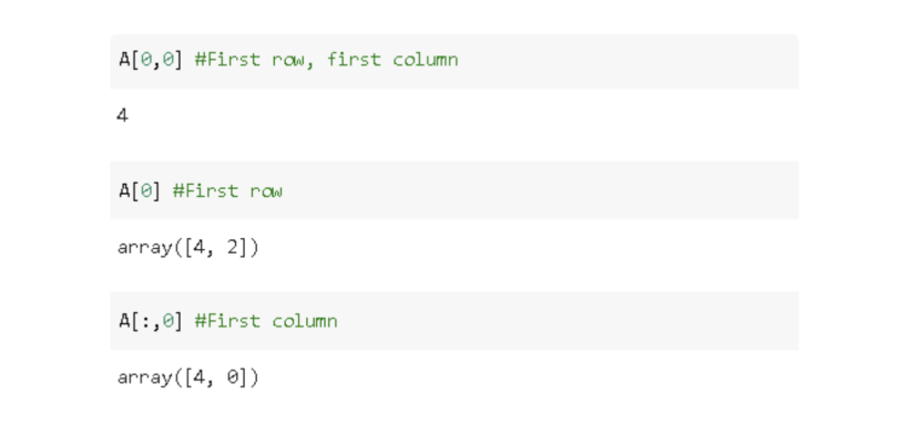
A 2x2 matrix has two rows and two columns. The index of rows and columns start with zero. For instance, the first row of A (row with index zero) is the array of [4, 2]. The first column of A is the array of [4, 0]. The element of the first row and first column is 4.
We can access individual rows, columns or elements with the following NumPy syntax:
1. Calculate the Dot Product Between the First Row of Matrix A and First Column of Matrix B
The first step is the dot product between the first row of A and the first column of B. The result of this dot product is the element of the resulting matrix at position [0, 0] (i.e. first row, first column.)

The resulting matrix, C, will have a (4*4) + (2*1) calculation at the first row and first column, so C[0, 0] = 18.
2. Calculate the Dot Product Between the First Row of Matrix A and Second Column of Matrix B
The next step is the dot product of the first row of A and the second column of B.

C will have a (4*0) + (2*4) at the first row and second column, so C[0,1] = 8.
3. Calculate the Dot Product Between the Second Row of Matrix A and First Column of Matrix B
First row A is complete, so we start on the second row of A and follow the same steps.

C will have a (0*4) + (3*1) at the second row and first column, so C[1,0] = 3.
4. Calculate the Dot Product Between the Second Row of Matrix A and Second Column of Matrix B
The final step is the dot product between the second row of A and the second column of B.

C will have a (0*0) + (3*4) at the second row and second column, so C[1,1] = 12.
We’ve now seen how it’s done step-by-step. All of these operations can also be done using an np.dot() operation:

Tips for Calculating Dot Product of a Matrix
As you may recall from vector dot products, two vectors must have the same length in order to have a dot product. Each dot product operation in a matrix multiplication must follow this rule. Dot products are done between the rows of the first matrix and the columns of the second matrix. Thus, the rows of the first matrix and columns of the second matrix must have the same length.
I want to emphasize an important point here: The length of a row is equal to the number of columns. Similarly, the length of a column is equal to the number of rows.
Consider the following matrix D:
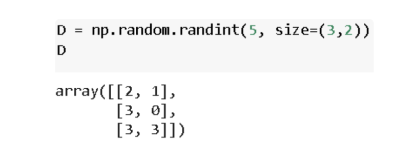
D has three rows and two columns, so it’s a 3x2 matrix. The length of a row is two, which is the number of columns, and the length of a column is three, which is the number of rows.
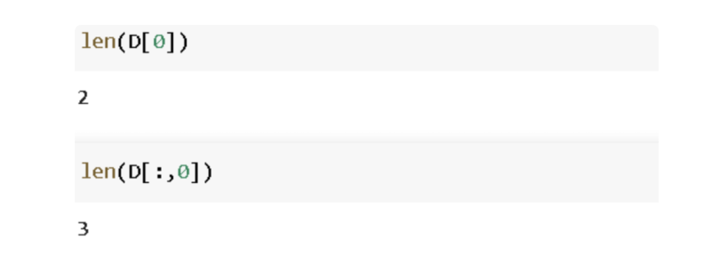
Length of a row and column for matrix D. | Image: Soner Yildirim
That’s the long explanation, but the point is that to be able to perform a matrix multiplication, the number of columns in the first matrix must be equal to the number of rows in the second matrix.
For instance, we can multiply a 3x2 matrix with a 2x3 matrix.
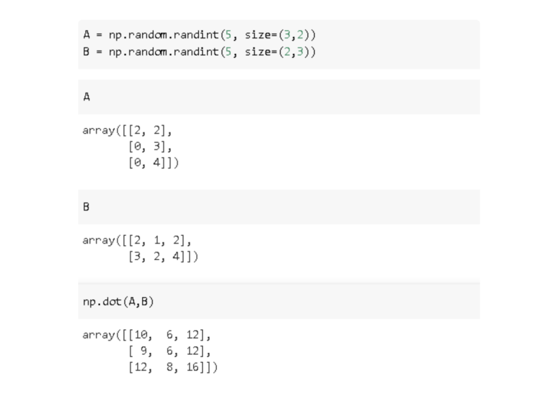
The shape of the resulting matrix will be 3x3 because we’re doing three dot product operations for each row of A, and A has three rows. An easy way to determine the shape of the resulting matrix is to take the number of rows from the first one and the number of columns from the second one:
- 3x2 and 2x3 multiplication returns 3x3.
- 3x2 and 2x2 multiplication returns 3x2.
- 2x4 and 4x3 multiplication returns 2x3.
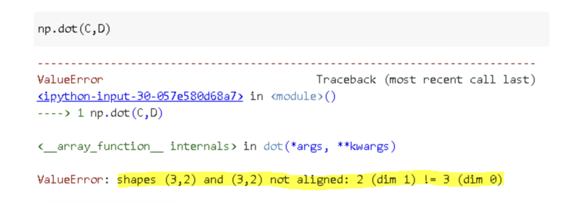
If the conditions we’ve been discussing are not met, matrix multiplication is impossible.
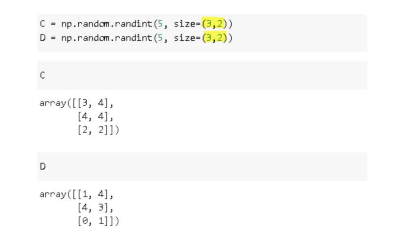
Consider the following matrices C and D. They both are 3x2 matrices:
If we try to multiply them, we will get the following value error:
We’ve now covered the basic, but very fundamental operations of linear algebra. Lots of matrix multiplication operations are done during the optimization process of machine learning models. Thus, it’s very important to also understand the basics, as well.
Frequently Asked Questions
How to do a dot product of a matrix?
A matrix product is done by calculating the dot product of the corresponding rows and columns between two matrices (also known as matrix multiplication). A dot product is the sum of the products of elements between two vectors, while a matrix product is the multiplication of two matrices to form a new matrix.
Two vectors must have the same length in order to have a dot product. Between two matrices, the rows of the first matrix and columns of the second matrix must have the same length to have a matrix product.
Is dot product just multiplication?
No, calculating the dot product of two vectors involves multiplying the corresponding elements at each position of the vectors, then adding the products of the elements together.
What is the purpose of the dot product of a matrix?
Machine learning models may use dot product and matrix product calculations to condense large amounts of data and facilitate computations, overall increasing model efficiency.


