Symmetric Matrix Properties and Applications: A Guide

A symmetric matrix is a matrix that is symmetric along the diagonal, which means Aᵀ = A, or in other words, the matrix is equal to its transpose. It’s an operator with the self-adjoint property. So, it’s important to think about a matrix as an operator and study its properties. While we can’t directly read off the geometric properties from the symmetry, we can find the most intuitive explanation of a symmetric matrix in its eigenvectors, which will give us a deeper understanding of the symmetric matrices.

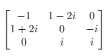
A trivial example is the identity matrix. A non-trivial example can be something like:

While the definition may be as simple as that, they contain a lot of probabilities and can mean different things. I’ll walk you through the important properties, explain them and then introduce the applications for a symmetric matrix.

The Hermitian matrix is a complex extension of the symmetric matrix, which means in a Hermitian matrix, all the entries satisfy the following:

The symmetric matrices are simply the Hermitian matrices but with the conjugate transpose being the same as themselves. Therefore, it has all the properties that a symmetric matrix has.

In data science, we mostly encounter matrices with real entries, since we are dealing with real-world problems. So, we’ll be exploring real cases of symmetric matrices.

Properties of a Symmetric Matrix

Three properties of symmetric matrices are introduced in this section. They are considered to be the most important because they concern the behavior of eigenvalues and eigenvectors of those matrices. Those are the fundamental characteristics, which distinguishes symmetric matrices from non-symmetric ones.

Property 1: Symmetric Matrices Have Real Eigenvalues.

This can be proved algebraically through a formal, direct proof, as opposed to induction, contradiction, etc. First, a quick explanation of eigenvalues and eigenvectors. The eigenvectors of matrix A are the vectors whose directions don’t change after A is applied to it. The direction is not changed, but the vectors can be scaled. This shows the non-triviality of this property. Real eigenvalues indicate stretching or scaling in the linear transformation, unlike complex eigenvalues, which don’t have a “size.”

The proportions that the vectors are scaled are called eigenvalues. We denote them by λ. Therefore, we have the relation Ax = λx. The proof is fairly easy, but it requires some knowledge of linear algebra. So, we will still go through it step by step.

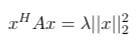
We’ll start with Ax = λx by the conjugate transpose of x, xᴴ, and we arrive at this equation:

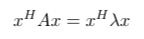
It’s important to note that λ is a scalar, which means the multiplication involving λ is commutative. Therefore, we can move it to the left of xᴴ.

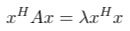
xᴴx is a Euclidean norm (or two-norm), which is defined as follows:

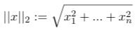
In a two-dimensional Euclidean space, it’s the length of a vector with coordinates (x₁, …, xₙ). We can then write equation1.3 as:

Since the conjugate transpose (operator H) works just like an ordinary transpose (operator T), we can use the property that xᴴA = (Ax)ᴴ.

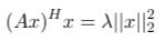
What does (Ax)ᴴ equal to? Here we will use the relation Ax = λx again, but this time (Ax)ᴴ will leave us the complex conjugate of λ, which we will denote it as λ with a bar.

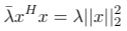
We have seen xᴴx before in equation 1.3. After substituting in the two-norm, which we can do because both λ_bar and xᴴx are scalars, we get this new equation:

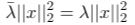
This leads to λ, and its complex conjugate being equal.

Only under one circumstance is equation 1.9 valid, which is when λ is real. And that finishes the proof.

More on Data ScienceRecursive SQL Expression Visually Explained

Property 2: Eigenvectors Corresponding to the Eigenvalues Are Orthogonal.

This is also a direct formal proof, but it’s simple. First, we need to recognize our target, which is the following:

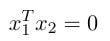
Consider a symmetric matrix A, where x₁ and x₂ are eigenvectors of A corresponding to different eigenvectors. Why we need this condition will be explained a bit later). Based on the definition of eigenvalues and symmetric matrices, we can get the following equations:

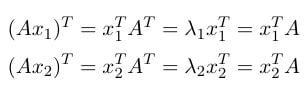
Now we need to approach equation 1.10. Let’s try to put x₁ and x₂ together. To do so, we multiply (Ax₁)ᵀ by x₁ᵀ on the left side:

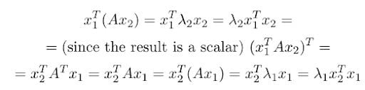
In equation 1.13 apart from the property of symmetric matrix, two other facts are used: 

1. The matrix multiplication is associative (vectors are n by 1 matrix).
2. Matrix-scalar multiplication is commutative meaning we can move the scalar freely. 

 Since dot production is commutative, this means x₁ᵀx₂ and x₂ᵀx₁ are the same things. We now have:

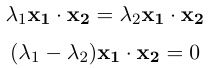
In the above equation, x₁∙x₂ denotes the dot product. If λ₁ ≠ λ₂, it must be the case that x₁∙x₂ = 0, which means those two eigenvectors are orthogonal. If λ₁ = λ₂, there are two different eigenvectors corresponding to the same eigenvalue. This can happen in an identity matrix. Since the eigenvectors are in the null space of (A-λI), which is denoted as N(A-λI), when one eigenvector corresponds to multiple eigenvectors, N(A-λI) has a dimension larger than one. In this case, we have infinite choices for those eigenvectors, and we can always choose them to be orthogonal.

There are cases where a real matrix has complex eigenvalues. This happens in rotation matrices. Why is that? Let Q be a rotation matrix. We know that the eigenvectors don’t change direction after being applied to Q. But if Q is a rotation matrix, how can x not change direction if x is a non-zero vector? The conclusion is that the eigenvector must be complex.

A rotation matrix R(θ) in the two-dimensional space is shown as follows:

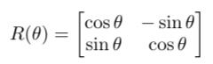
R(θ) rotates a vector counterclockwise by an angle θ. It is a real matrix with complex eigenvalues and eigenvectors.

Property 3: Symmetric Matrices Are Always Diagonalizable. 

This is known as the spectral theorem. It is also related to the other two properties of symmetric matrices. The name of this theorem might be confusing. In fact, the set of all the eigenvalues of a matrix is called a spectrum. Also, we can think about it like this: the eigenvalue-eigenvector pairs tell us in which direction a vector is distorted after the given linear transformation.

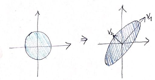
This is shown in the following figure. After transformation, in the direction of v₁, the figure is stretched a lot. But in the direction of v₂, it’s not stretched very much.

A matrix that is diagonalizable means there exists a diagonal matrix D (all the entries outside of the diagonal are zeros), such that P⁻¹AP = D, where P is an invertible matrix. We can also say that a matrix is diagonalizable if the matrix can be written in the form A = PDP⁻¹.

The decomposition is unique up to the permutation of the entries on the diagonal in D and the scalar multiplication of the eigenvectors in P. We also need to note that the diagonalization is equivalent to finding eigenvectors and eigenvalues, no matter if the matrix is symmetric or not. However, for a non-symmetric matrix, D doesn’t have to be an orthogonal matrix,

Those two definitions are equivalent, but they can be interpreted differently. This decomposition makes raising the matrix to power very handy. The second one, A = PDP⁻¹, tells us how A can be decomposed. Meanwhile, the first one, P⁻¹AP = D, is the one that tells us A can be diagonalized. It tells us that it is possible to align the standard basis given by the identity matrix with the eigenvectors. The orthogonality of the eigenvectors, which is shown in property two, enables this. 

The phrase “align the standard basis with the eigenvectors” sounds abstract. We need to think about this: What does matrix transformation do to the basis? A matrix consisting of basis α = {v₁, …, vₙ}, with those vectors in the column, transforms a vector x from the standard basis to the coordinate system formed by basis α.We denote this matrix by Aα. Therefore, in the process of the diagonalization P⁻¹AP = D, P sends a vector from the standard basis to the eigenvectors, A scales it, and then P⁻¹ sends the vector back to the standard basis. From the perspective of the vector, the coordinate system is aligned with the standard basis with the eigenvectors.

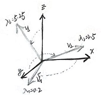
This alignment is shown in the figure above. The matrix used in this example is:

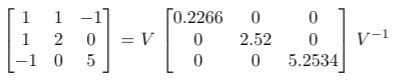
Where V is the matrix with eigenvectors of length one as the columns, each of them corresponds to the eigenvalues in the diagonal matrix. As for the calculation, we can let eig in MATLAB do the work.

This property follows the spectral theorem directly, which dictates that if A is Hermitian, there exists an orthonormal basis of V consisting of eigenvectors of A. Each eigenvector is real.

The theorem directly points out a way to diagonalize a symmetric matrix. To prove the property directly, we can use induction on the size or dimension of the matrix. The basic idea of the proof is that the base case, where A is a one-by-one matrix, is trivial. Assume that the n-1-by-n-1 matrix is diagonalizable, meaning it has n-1 independent eigenvectors). We can find another eigenvector in n-dimensional space, which is orthogonal to those n-1 dimensional eigenvectors. Thus, the n-by-n matrix is also diagonalizable.

How to Identify the Definiteness of a Symmetric Matrix

When are those properties useful? Even before the formal study of matrices, they have been used for solving systems of linear equations for a long time. Think about the matrices as operators. The information of the linear equations is stored in those operators, meaning matrices can be used to study the behavior of functions.

Beyond symmetry, an even better property matrix can have is positive-definiteness. If a symmetric (or Hermitian) matrix is positive-definite, all of its eigenvalues are positive. If all of its eigenvalues are non-negative, then it is a semi-definite matrix. For a matrix to be positive-definite, it’s required to be symmetrical because of property one. Since it only makes sense to ask whether a number is positive or negative, how large it is or when it is real.

Symmetric vs. Skew-Symmetric Matrix

A symmetric matrix is a matrix equal to its transpose. In contrast, a skew-symmetric (or antisymmetric or antimetric) matrix is one that is opposite to its transpose, or when its transpose equals its negative. 

In a skew-symmetric matrix, the condition Aᵀ = -A is met, plus all main diagonal entries are zero and the matrix’s trace equals zero. The sum of two skew-symmetric matrices, as well as a scalar multiple of a skew-symmetric matrix, will always be skew-symmetric.

Applications of Symmetric Matrices

Statistics

In statistics and multivariate statistics, symmetric matrices can be used to organize data, which simplifies how statistical formulas are expressed, or presents relevant data values about an object. Symmetric matrices may be applied for statistical problems covering data correlation, covariance, probability or regression analysis.

Machine Learning and Data Science 

Symmetric matrices, such as Hessian matrices and covariance matrices, are often applied in machine learning and data science algorithms to optimize model processing and output. A matrix can help algorithms effectively store and analyze numerical data values, which are used to solve linear equations. 

Engineering and Robotics

Symmetrical matrices can provide structure for data points and help solve large sets of linear equations needed to calculate motion, dynamics or other forces in machines. This can be helpful for areas in control system design and optimization design of engineered systems, as well as for solving engineering problems related to control theory. 

How to Apply a Symmetric Matrix

A good application of a symmetric matrix is the Hessian matrix. We will use this as an example to demonstrate using matrices for analyzing function behavior. When we try to find a local extreme, it’s always good to find out that the Hessian is positive definite. The Hessian is a matrix consisting of the second partial derivatives of a real function. Formally, let f: ℝⁿ ➝ℝ be a function, the Hessian is defined as

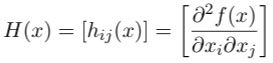
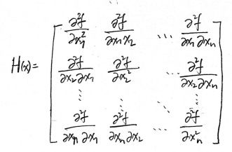
And we call H(x) the Hessian of f, which is an n-by-n matrix. In definition 1.18, the Hessian is written very compactly. It is the same thing as

How does this affect function behavior? We will look at one super simple example. Consider the function f(x, y) = y²-x². The Hessian is computed as follows:

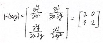
It can also be computed using the function hessian in MATLAB. Since it’s a diagonal matrix and the trace (sum of the entries on the diagonal) equals the sum of eigenvectors, we can immediately see that one of the eigenvalues is two and another one is negative two. They correspond to the eigenvectors v₁ = [1, 0]ᵀ and v₂ = [0, 1]ᵀ. This matrix is symmetric but not positive definite. Therefore, there’s no local extreme in the whole ℝ². We can only find a saddle point on point x=0, y=0. This means in the direction of v₁, where the eigenvalue is positive, the function increases. But in the direction of v₂, where the eigenvalue is negative, the function decreases. The image of the function is shown below:

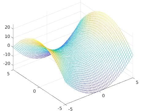
The image is generated using MATLAB with the following code.

clc; clear; close all

xx = -5: 0.2: 5;
yy = -5: 0.2: 5;

[x, y] = meshgrid(xx, yy);

zz = x.^2 - y.^2;

figure
mesh(x, y, zz)
view(-10, 10)

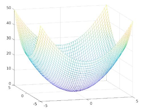
Now, we flip the sign and change the function into f(x, y) = x² + y². The eigenvectors remain the same, but all the eigenvectors become positive. This means, in both the direction of v₁ and the direction of v₂, the function grows. Therefore, the local minimum can be found at x=0, y=0, f(x,y) = 0. This is also the global minimum. The graph looks like this:

More on Data ScienceUnderstanding and Building Neural Network (NN) Models

Symmetric Matrix Advantages

Matrices have wide-usage in numerous fields. When dealing with matrices, the concepts of positive-definiteness, eigenvectors, eigenvalues and symmetric matrices are often encountered. 

Frequently Asked Questions