A confusion matrix in Python is an N x N table used to assess the performance of a classification model. It compares the predicted labels with the actual labels, helping to visualize how well the model is performing by showing the number of true positives, true negatives, false positives and false negatives. This allows for a deeper understanding of the model’s strengths and weaknesses.
What Is a Confusion Matrix?
A confusion matrix is used to evaluate the performance of a classification algorithm. It’s an N x N grid, where N is the number of outcomes. It helps you understand how well the classification algorithm is performing and where errors originate.
To help us understand the confusion matrix, we’ll use an example from the Economic Times about Covid RT-PCR test results.
“The RT-PCR test is more sensitive when it comes to gene testing and, hence, more accurate,” according to the article.
The terms “sensitive” and “accurate” are key performance metrics that can be calculated from the values within a confusion matrix. Let’s look at the RT-PCR test as a classification model. It predicts whether the patient is infected, and the confusion matrix is used to evaluate its performance.
How Does the Confusion Matrix Work?
The confusion matrix helps you understand how well your classification model is performing and identifies where errors occur. So, what does that mean?
Let’s say that you have a classification model that is 95 percent accurate. This means that out of 100 records, 95 records have predicted values the same as actual values, i.e. the model predicts 95 records correctly.
The same model also predicted five records incorrectly, i.e. the error is 5 percent. However, from the statement about accuracy, you have no idea where those 5 percent errors occurred or their origin.
This is where the confusion matrix comes in.
How to Create a Confusion Matrix
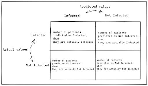
You can create it with predicted values on one axis and actual values on another. Then, you need to fill in the count of predicted and actual values in the respective cells, as shown below.
Let’s continue with the RT-PCR test example to understand the concept in depth. Suppose you conducted an RT-PCR test of 10 patients, where the test answered the question: Is the patient infected?
There were two outcomes of the test: YES or NO. Below was the list of actual and predicted results.
actual = [NO, YES, YES, YES, YES, NO, NO, YES, YES, YES]
predicted = [YES, NO, YES, NO, NO, YES, NO, YES, YES, YES]
Since there are only two outcomes, the confusion matrix is 2 x 2.
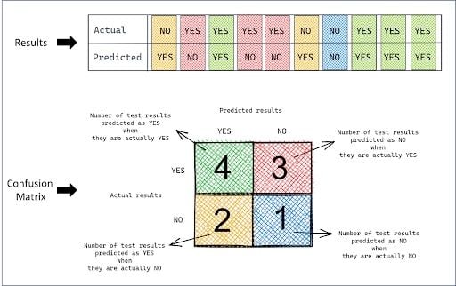
Simply compare the predicted values with the actual values and take its count to fill in corresponding cells in the confusion matrix.
Confusion Matrix Terms to Know
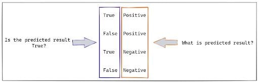
Although the above picture is self-explanatory, each cell of the confusion matrix has a distinct scientific terminology, as shown below.
1. True Positive (TP)
A true positive (TP) is when the model predicts a positive result, and the actual result is also positive. The location of this value (e.g., first row, first column) depends on the specific layout convention of the confusion matrix you are using.
2. True Negative (TN)
A true negative (TN) occurs when the test result is predicted as NO and it is actually NO, i.e. negative. This means the prediction is true. The cell in the second row, second column represents this.
3. False Positive (FP)
A false positive (FP) occurs when the test result is predicted as YES, i.e. positive, when it is actually NO. This means the prediction is false. The cell in the second row, first column represents this.
4. False Negative (FN)
A false negative (FN) occurs when the test result is predicted as NO, i.e. Negative, but it is actually YES. This means the prediction is false. The cell in the first row, second column represents this.
Here is a quick-tip on how to read it.
All the false results, such as false positive and false negative, are the errors in the test. The confusion matrix can help you to quantify these errors.
Now you can tell how many times, and in which situations your classification model (RT-PCR test in this example) failed to predict correctly. In statistics, false positive (FP) is a Type I error, and false negative (FN) is a Type II error.
Generally, a false negative is considered a dangerous error in medical sciences.
A Type II error in the RT-PCR test example occurs when the patient is predicted as negative, when it’s actually positive. Based on the test results, if this patient did not take enough precautions, Covid-19 could spread to a wider population.
To evaluate the performance of the classification model, one should consider all the cells from the confusion matrix.
Confusion Matrix Metrics
Further calculations from the confusion matrix can capture the effects of all correct and incorrect predictions.
Below are the commonly inferred confusion matrix metrics:
1. Accuracy
A confusion matrix helps you to understand how often your classification model is correct. Accuracy measures the proportion of total predictions that were correct. It tells you how often your model made the right prediction out of all its predictions.
Mathematically, accuracy can be calculated by dividing all the true values, i.e. number of all the true positive (TP) and true negative (TN) results, by the total number of results.
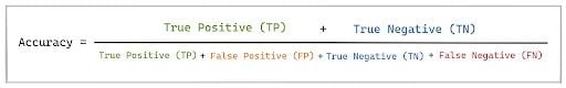
In our example, accuracy is (4+1)/(4+1+3+2) = 0.5, which means only 50 percent of the time the model makes a correct prediction.
Accuracy may not be a good metric when the data set contains a different number of positive and negative results.
For example, there are eight non-infected patients and only two infected patients in the data set. Now, suppose your model predicted all the patients as non-infected. The confusion matrix in this scenario will have TP = 0, FP = 0, TN = 8 and FN = 2.
The accuracy in this case will be (8+0)/(0+0+8+2) = 0.8. Although the accuracy is 80 percent, this model is very poor, as it predicted all the infected patients as non-infected, which gives rise to a false negative, i.e. a Type II error.
Accuracy only captures the share of correctly predicted results in the total number of results. It doesn’t account for any misclassifications or false results. So, with the accuracy of 80 percent, you don’t know how the remaining 20 percent is distributed between false negative and false positive.
Therefore, we need other metrics to evaluate the performance of the classification model.
2. Sensitivity
This metric helps you understand how often the model predicts a correct yes. It’s a true positive rate, which is calculated by dividing the number of true positive results by the total number of actual positive results.
Mathematically, it’s calculated as:
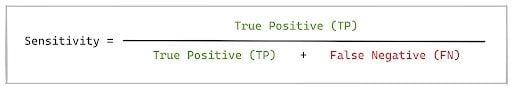
Therefore, when the sensitivity is high, there are fewer false negative results.
In the RT-PCR test example, sensitivity is calculated as 4/(4+3) = 0.57. This means the test has a sensitivity of 57 percent. So, out of all the patients who were actually infected with Covid-19, the RT-PCR test correctly predicted only 57 percent.
Sensitivity and recall are interchangeable terms, and both are used often in statistics. However, while sensitivity and recall are mathematically identical (TP/(TP+FN)), their usage often depends on the field. In medical or scientific contexts, you will commonly see sensitivity paired with specificity (the true negative rate). In machine learning and data science, recall is more frequently used and typically paired with precision (the positive predictive value).
3. Specificity
Specificity is the opposite of sensitivity, as it is the true negative rate. It’s calculated by dividing the number of true negatives by the total number of actual negative results.
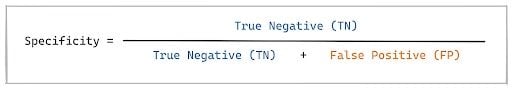
This metric helps you understand how often the classification model predicts a NO, and it returns an actual NO.
In the RT-PCR test example, specificity is calculated as 1/(1+2) = 0.333. This means the test has a specificity of 33.3 percent. So, out of all the patients who weren’t infected with Covid, the RT-PCR test only correctly predicted 33 percent of them.
4. Precision
Precision helps you to understand how often a model correctly predicts a positive result. Ideally, a precision of one or 100 percent indicates that whenever the model predicts positive, it’s 100 percent correct.
The precision is the number of true positive results divided by the total number of positive results:
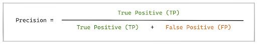
To get precision of 100 percent or one, false positive value should become zero. This means that none of the negative values get predicted as positive.
In the RT-PCR test example, you can get precision as 4/(4+2) = 0.666. It indicates that, whenever this classification model predicts the patient as infected, it’s only correct 66.6 percent of the time.
Well, you might be wondering how to calculate these metrics in a real project. The majority of machine learning libraries have methods that calculate all these metrics in just one line of code.
How to Create a Confusion Matrix in Python
When you utilize Python to build a classification model, the machine learning library scikit-learn has the built-in function confusion_matrix to create a confusion matrix.
Let’s transform our RT-PCR test example and replace every YES with 1 and NO with 0 to use this function.
actual = [0, 1, 1, 1, 1, 0, 0, 1, 1, 1]
predicted = [1, 0, 1, 0, 0, 1, 0, 1, 1, 1]
from sklearn import metrics
confusion_matrix = metrics.confusion_matrix(actual, predicted)
display(confusion_matrix)
#Output
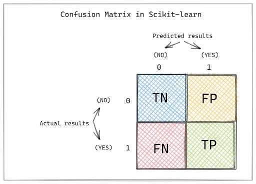
array([[1, 2],
[3, 4]], dtype=int64)The output matrix looks slightly different from the confusion matrix you saw earlier in this article. That’s because scikit-learn has a different arrangement of predicted and actual values in the confusion matrix.
Therefore, the confusion matrix created using scikit-learn follows the structure below.
How to Use Seaborn to Visualize a Confusion Matrix in Python
You can also visualize this matrix using data visualization library Seaborn as shown below.
import seaborn as sns
sns.heatmap(confusion_matrix, annot=True)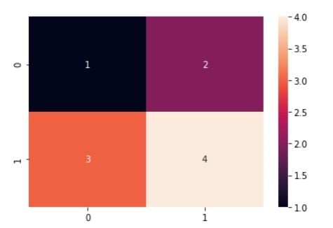
How to Display Metrics for a Confusion Matrix in Python
Although you can understand the TP, TN, FP and FN from this confusion matrix, the real question is still not answered: How do I get metrics such as precision, recall and accuracy using Python?
And the answer lies again in the same scikit-learn library. Scikit-learn offers the built-in functions accuracy_score, precision_score, recall_score to answer your questions:
print(f"Accuracy = {metrics.accuracy_score(actual, predicted)}")
print(f"Precision = {metrics.precision_score(actual, predicted)}")
print(f"Recall = {metrics.recall_score(actual, predicted)}")

#Output

Accuracy = 0.5
Precision = 0.6666666666666666
Recall = 0.5714285714285714
You can see this output matches exactly with the one you calculated manually.
There are multiple metrics to evaluate the performance of a classification model but choosing the right one depends on the problem you are solving. Generally, accuracy is used to understand if the model is good or bad, but when the data set is unbalanced it’s always better to look at other metrics, as well.
Frequently Asked Questions
What is a confusion matrix?
A confusion matrix is a table used to evaluate a classification model's performance. It is an N x N grid (where N is the number of outcomes) that summarizes the predicted results versus the actual results, helping users understand where a model makes errors.
What are the four key terms in a confusion matrix?
The four key terms of a confusion matrix are:
- True Positive (TP): The model correctly predicted a positive outcome.
- True Negative (TN): The model correctly predicted a negative outcome.
- False Positive (FP): The model incorrectly predicted a positive outcome when it was actually negative. This is also known as a Type I error.
- False Negative (FN): The model incorrectly predicted a negative outcome when it was actually positive. This is also known as a Type II error.
What are the four metrics derived from a confusion matrix?
The four main metrics derived from a confusion matrix include:
- Accuracy: Measures the overall correctness of the model. It is the ratio of correctly predicted outcomes (True Positives + True Negatives) to the total number of outcomes.
- Sensitivity (Recall): Measures the model's ability to correctly identify all actual positive cases. It is the ratio of true positives to all actual positive cases (True Positives + False Negatives).
- Specificity: Measures the model's ability to correctly identify all actual negative cases. It is the ratio of true negatives to all actual negative cases (True Negatives + False Positives).
- Precision: Measures how reliable the model is when it predicts a positive outcome. It is the ratio of true positives to all predicted positive cases (True Positives + False Positives).