Singular Value Decomposition (SVD) Algorithm Explained

Singular value decomposition (SVD) is a matrix factorization method that generalizes the eigendecomposition of a square matrix (n x n) to any matrix (n x m).

SVD is similar to principal component analysis (PCA), but it’s more general. PCA assumes that the input is a square matrix, SVD doesn’t have this assumption. 

SVD Algorithm Mathematics

The general formula for SVD is:

M=UΣVᵗ, where:

• M is the original matrix we want to decompose.
• U is the left singular matrix (columns are left singular. vectors). U columns contain eigenvectors of matrix MMᵗ.
• Σ is a diagonal matrix containing singular eigenvalues.
• V is a right singular matrix (columns are right singular vectors). V columns contain eigenvectors of matrix MᵗM.

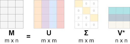
SVD is more general than PCA. SVD can handle matrices with a different number of columns and rows. PCA formula is M=𝑄𝚲𝑄ᵗ, which decomposes matrix into orthogonal matrix 𝑄 and diagonal matrix 𝚲. Simply this could be interpreted as:

• Change of the basis from standard basis to basis 𝑄 (using 𝑄ᵗ).
• Applying transformation matrix 𝚲, which changes length not direction, as this is a diagonal matrix.
• Change of the basis from basis 𝑄 to standard basis (using 𝑄).

SVD does similar things, but it doesn’t return to the same basis from which we started transformations. It couldn’t do it because our original matrix M isn’t a square matrix. 

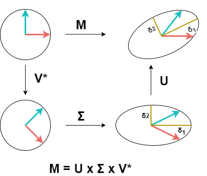
SVD does the following steps:

• Change of the basis from standard basis to basis V (using Vᵗ). 
• Apply transformation described by matrix Σ. This scales our vector in basis V.
• Change of the basis from V to basis U. Because our original matrix M isn’t square, matrix U can’t have the same dimensions as V and we can’t return to our original standard basis.

There are numerous variants of SVD and ways to calculate SVD. I’ll show just a few of the ways to calculate it.

More on AIMath for AI: A Guide

3 Ways to Calculate SVD

If you want to try coding examples yourself use this notebook which has all the examples from this post.

1. Power Iteration

Power iteration starts with b₀, which might be a random vector. At every iteration this vector is updated using following rule:

First we multiply b₀ with original matrix A (Abₖ) and divide the result with the norm (||Abₖ||). We’ll continue until the result has converged, in other words, updates are less than the threshold.

The power method has few assumptions:

• b₀ has a nonzero component in the direction of an eigenvector associated with the dominant eigenvalue. Initializing b₀ randomly minimizes possibility that this assumption is not fulfilled.
• Matrix A has a dominant eigenvalue that must be greater in magnitude than other eigenvalues.

These assumptions guarantee that the algorithm converges to a reasonable result. The smaller the difference between dominant eigenvalue and second eigenvalue, the longer it might take to converge.

I’ve created an example that also finds the eigenvalue. As you can see, the core of this function is power iteration.

def eigenvalue(A, v):
    # uses property A @ eigenvector = eigenvalue @ eigenvector =>
    # eigenvalue = (A @ eigenvector) / eigenvector
    val = A @ v / v
    return val[0]

def svd_power_iteration(A):
    n, d = A.shape
    #create original normal vector v which is used to approximate dominant eigenvalue
    v = np.ones(d) / np.sqrt(d)
    ev = eigenvalue(A, v)
    while True:
        #these two lines are basically the core of power iteration
        Av = A @ v
        v_new = Av / np.linalg.norm(Av)
        ev_new = eigenvalue(A, v_new)
        #break if new eigenvalue is not much different from previous
        if np.abs(ev - ev_new) < 0.01:
            break
        v = v_new
        ev = ev_new
    return ev_new, v_new

SVD Algorithm Power Iteration Example

For a simple example, we’ll use the beer data set. We’ll construct a covariance matrix and try to determine the dominant singular value of the data set.

#construct data 
df=pd.read_csv('data/beer_dataset.csv')
X = np.array([df['Temperatura Maxima (C)'],
              df['Consumo de cerveja (litros)']]).T
C = np.cov(X, rowvar=False)
eigen_value, eigen_vec = svd_power_iteration(C)

We can plot the dominant eigenvector with original data.

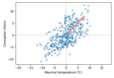
As you can see from the plot, this method found the dominant singular value/eigenvector. It looks like it’s working. You’ll see in the notebook that results are very close to results from the SVD implementation provided by numpy. Next, we’ll see how to get more than just first dominant singular values.

More on Artificial IntelligenceExplore Built In’s AI Coverage

2. Iteration for N Singular Values

To get more than just the most dominant singular value from a matrix, we could still use power iteration. We’ll implement a new function that uses our previous svd_power_iteration function. Finding the first dominant singular value is easy. We could use the previously mentioned function. But how do you find the second singular value?

We should remove the dominant direction from the matrix and repeat, finding the most dominant singular value. To do that, we could subtract previous eigenvector(s) component(s) from the original matrix using singular values and left and right singular vectors that we’ve already calculated:

A_next = A-(singular_value₁)(u₁)(v₁)ᵗ

Here is example code with minor modifications for calculating multiple eigenvalues/eigenvectors.

def svd(A, k=None, epsilon=1e-10):
    """returns k dominant eigenvalues and eigenvectors of matrix A"""
    A = np.array(A, dtype=float)
    n, m = A.shape
        
    svd_so_far = []
    if k is None:
        k = min(n, m)

    for i in range(k):
        matrix_for_1d = A.copy()
        #ubtract previous eigenvector(s) component(s)
        for singular_value, u, v in svd_so_far[:i]:
            matrix_for_1d -= singular_value * np.outer(u, v)
        #here also deal with different dimensions, 
        #otherwise shapes don't match for matrix calculus
        if n > m:
            _, v = svd_dominant_eigen(matrix_for_1d, epsilon=epsilon)  # next singular vector
            u_unnormalized = A @ v
            sigma = np.linalg.norm(u_unnormalized)  # next singular value
            u = u_unnormalized / sigma
        else:
            _, u = svd_dominant_eigen(matrix_for_1d, epsilon=epsilon)  # next singular vector
            v_unnormalized = A.T @ u
            sigma = np.linalg.norm(v_unnormalized)  # next singular value
            v = v_unnormalized / sigma

        svd_so_far.append((sigma, u, v))

    singular_values, us, vs = [np.array(x) for x in zip(*svd_so_far)]
    return singular_values, us.T, vs

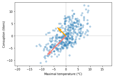
When we apply this to our beer data set, we get two eigenvalues and eigenvectors.

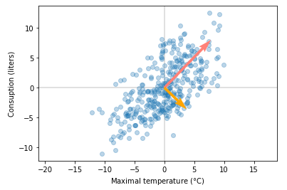
This example works also with matrices, which have more columns than rows or more rows than columns. Results are comparable to numpy SVD implementation. Here is one example:

mat = np.array([[1,2,3],
                [4,5,6]])
u, s, v = np.linalg.svd(mat, full_matrices=False)
values, left_s, rigth_s = svd(mat)
np.allclose(np.absolute(u), np.absolute(left_s))
#True
np.allclose(np.absolute(s), np.absolute(values))
#True
np.allclose(np.absolute(v), np.absolute(rigth_s))
#True

To compare our custom solution results with the numpy SVD implementation, we take absolute values because signs in the matrices might be opposite. It means that vectors point opposite directions but are still on the same line, and thus, are still eigenvectors.

Now that we have found a way to calculate multiple singular values/singular vectors, we might ask, could we do it more efficiently?

3. Block Version of the Power Method

This version  is also known as simultaneous power iteration or orthogonal iteration. The Idea behind this version is pretty straightforward. For starters, other eigenvectors are orthogonal to the dominant eigenvector. The power method forces the second vector to become orthogonal to the first one. The algorithm then converges to two or more different vectors.

Each step we multiply A not just by just one vector, but by multiple vectors which we put in a matrix Q. At each step we’ll normalize the vectors using QR Decomposition. QR decomposition decomposes matrix into following components:

A=QR, where

• A is the original matrix we want to decompose
• Q is the orthogonal matrix
• R is the upper triangular matrix

If the algorithm converges, then Q will be eigenvectors and R eigenvalues. Here is example code:

def svd_simultaneous_power_iteration(A, k, epsilon=0.00001):
    #source https://mlwiki.org/index.php/Power_Iteration
    #adjusted to work with n<m and n>m matrices
    n_orig, m_orig = A.shape
    if k is None:
        k=min(n_orig,m_orig)
    A_orig=A.copy()
    if n_orig > m_orig:
        A = A.T @ A
        n, m = A.shape
    elif n_orig < m_orig:
        A = A @ A.T
        n, m = A.shape
    else:
        n,m=n_orig, m_orig
        
    Q = np.random.rand(n, k)
    Q, _ = np.linalg.qr(Q)
    Q_prev = Q
    #this part does the block power iteration
    for i in range(1000):
        Z = A @ Q
        Q, R = np.linalg.qr(Z)
        err = ((Q - Q_prev) ** 2).sum()
        Q_prev = Q
        if err < epsilon:
            break
            
    singular_values=np.sqrt(np.diag(R)) 
    #deal with different shape input matrices
    if n_orig < m_orig: 
        left_vecs=Q.T
        #use property Values @ V = U.T@A => V=inv(Values)@U.T@A
        right_vecs=np.linalg.inv(np.diag(singular_values))@left_vecs.T@A_orig
    elif n_orig==m_orig:
        left_vecs=Q.T
        right_vecs=left_vecs
        singular_values=np.square(singular_values)
    else:
        right_vecs=Q.T
        #use property Values @ V = U.T@A => U=A@V@inv(Values)
        left_vecs=A_orig@ right_vecs.T @np.linalg.inv(np.diag(singular_values))

    return left_vecs, singular_values, right_vecs

From the code we could see that calculating singular vectors and values is  a small part of the code. Much of the code is dedicated to dealing with different shaped matrices.

If we apply this function to the beer data set, we should get similar results as we did with  the previous approach.

Eigenvectors point opposite directions compared to the previous version, but they are on the same (with a small error) line, and thus, are the same eigenvectors. In the notebook I have examples that compares output with numpy SVD implementation.

Applications of SVD Algorithm

The SVD algorithm has a number of applications in artificial intelligence and machine learning. It is a great tool for dimensionality reduction and finding components with most variance from the data. For that reason SVD is used for the following applications:

1. Data compression: SVD reduces high-dimensional data to lower dimensions while preserving important features. For example, reducing the size of a photo file.
2. Image processing: SVD could be used for noise reduction if you have partially corrupted images and facial recognition.
3. Recommendation systems: SVD helps in collaborative filtering for personalized recommendations.
4. Natural language processing: SVD can be used in latent semantic analysis for text mining and information retrieval.
5. Machine learning: SVD is used in dimensionality reduction techniques like PCA, which help make model training faster and results more accurate.

There are many more applications where SVD is being used. Its relative simplicity makes it easy and resource efficient to use.

More on Machine LearningAll Machine Learning Models Explained

Understanding the SVD Algorithm

To calculate the dominant singular value and singular vector, we could use the  power iteration method. This method could be adjusted for calculating n-dominant singular values and vectors. For simultaneous singular value decomposition, we could use the block version of power iteration. These methods aren’t the fastest nor the most stable methods, but they are great sources for learning how the SVD algorithm works

Frequently Asked Questions