

A covariance matrix is a square matrix of elements that represent the covariance values between each pair of variables in a data set or given vector.
Covariance Matrix Definition
A covariance matrix displays the covariance values of each pair of variables in multivariate data. These values show the distribution magnitude and direction of multivariate data in a multidimensional space, and can allow you to gather information about how data spreads among two dimensions.
When dealing with statistics and machine learning problems, one of the most frequently encountered concepts is covariance. While most of us know that variance represents the variation of values in a single variable, we may not be sure what covariance means. However, understanding covariance can provide more information to help you solve multivariate problems. Most of the methods for preprocessing or predictive analysis also depend on the covariance, including, multivariate outlier detection, dimensionality reduction and regression.
I’m going to explain five things that you should know about covariance. Instead of just focusing on the definition, we will try to understand covariance from its formula.
What Is Variance and Covariance?
In order to better understand covariance, we need to first go over variance. Variance explains how the values vary in a variable. It depends on how far the values are from each other.
Take a look at formula one to understand how variance is calculated.
Variance Formulas
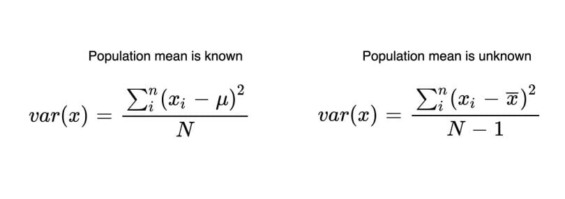
In the formula, each value in the variable subtracts from the mean of that variable. After the differences are squared, it gets divided by the number of values (N) in that variable. What happens when the variance is low or high? As you can see in the image below, what happens when the variance value is low or high.

Covariance Formulas
Now, let’s look at the covariance formula. It’s as simple as the variance formula. Unlike variance, however, covariance is calculated between two different variables. Its purpose is to find the value that indicates how these two variables vary together. In the covariance formula, the values of both variables are multiplied by taking the difference from the mean. You can see this in the formula below.
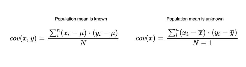
The only difference between variance and covariance is that you’re using the values and means of two variables instead of one in covariance. Now, let’s take a look at the second thing that you should know.
There are two different formulas for when the population is known and unknown. When we work on sample data, we often don’t know the population mean. We only know the sample mean. That’s why we should use the formula with N-1. When we have the entire population of the subject, you can use N.
What Is a Covariance Matrix?
The second thing that you should know about is the covariance matrix. Because covariance can only be calculated between two variables, covariance matrices stand for representing covariance values of each pair of variables in multivariate data. Also, the covariance between the same variables equals the variance. So, the diagonal shows the variance of each variable. Suppose there are two variables, x and y, in our data set. The covariance matrix should look like the formula below.
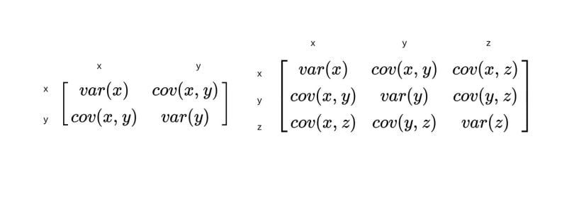
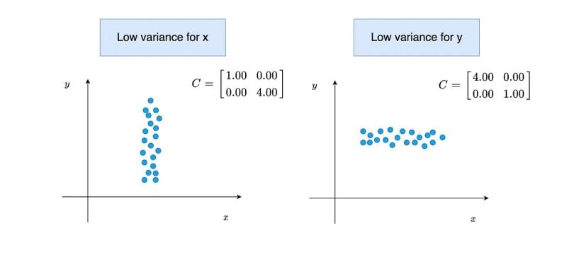
A symmetric matrix shows covariances of each pair of variables. These values in the covariance matrix show the distribution magnitude and direction of multivariate data in a multidimensional space. By controlling these values, we can gather information about how data spreads among two dimensions.
Positive, Negative and Zero States of the Covariance
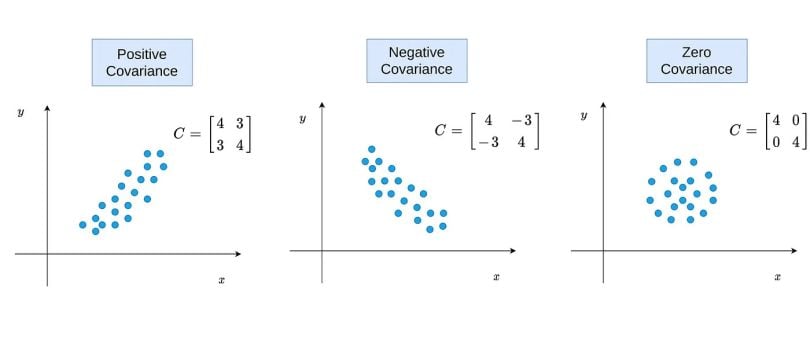
The third thing that you should know about covariance is its positive, negative and zero states. We can go over the formula to understand it. When Xi-Xmean and Yi-Ymean are both negative or positive at the same time, multiplication returns a positive value. If the sum of these values is positive, covariance returns as positive. This means variable X and variable Y vary in the same direction. In other words, if a value in variable X is higher, it is expected to be high in the corresponding value in variable Y, too. In short, there is a positive relationship between them. If there is a negative covariance, this is interpreted in the opposite direction. That is, there is a negative relationship between the two variables.
The covariance can only be zero when the sum of products of Xi-Xmean and Yi-Ymean is zero. However, the products of Xi-Xmean and Yi-Ymean can be near-zero when one or both are zero. In such a scenario, there aren’t any relations between variables. To understand it clearly, you can see the following image.
In another possible scenario, we can have a distribution like in the image below. This happens when the covariance is near zero and the variance of variables are different.
Size of a Covariance Value
Unlike correlation, covariance values do not have a limit between -1 and 1. Therefore, it could be wrong to conclude that there might be a high relationship between variables when the covariance is high. The size of covariance values depends on the difference between values in variables. For instance, if the values are between 1,000 and 2,000 in the variable, it’s possible to have high covariance. However, if the values are between one and two in both variables, it’s possible to have a low covariance. Therefore, we can’t say the relationship in the first covariance matrix example is stronger than the second. The covariance stands only for the variation and relation direction between two variables. You can understand it from the image below.
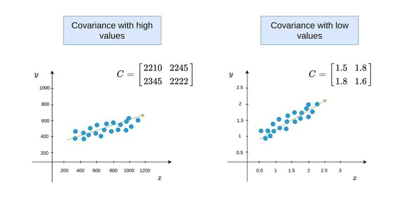
Although the covariance in the first figure is very large, the relationship can be higher or the same in the second figure. The values in the above image are given as examples; they aren’t from any data set and aren’t true values.
Eigenvalues and Eigenvectors of Covariance Matrix
What do eigenvalues and eigenvectors tell us? These are essential components of the covariance matrix. The methods that require a covariance matrix to find the magnitude and direction of the data points use eigenvalues and eigenvectors. For example, the eigenvalues represent the magnitude of the spread in the direction of the principal components in principal component analysis (PCA).
In the image below, the first and second plots show the distribution of points when the covariance is near zero. When the covariance is zero, eigenvalues will be directly equal to the variance values. The third and fourth plots represent the distribution of points when the covariance is different from zero. Unlike the first two, eigenvalues and eigenvectors should be calculated for these two.
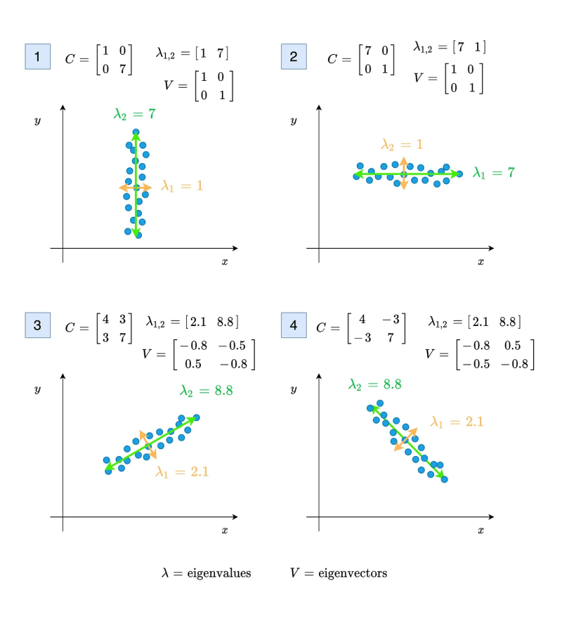
As you can see in the above image, the eigenvalues represent the magnitude of the spread for both variables x and y. The eigenvectors show the direction. It’s possible to find the angle of propagation from the arccosine of the value v[0,0] when the covariance is positive. If the covariance is negative, the cosine of the value v[0,0] gives the spread direction.
How do you find eigenvalues and eigenvectors from the covariance matrix? You can find both eigenvectors and eigenvalues using NumPy in Python. First thing you should do is find the covariance matrix using the method numpy.cov(). After you’ve found the covariance matrix, you can use the method numpy.linalg.eig(M) to find eigenvectors and eigenvalues.
Applications of the Covariance Matrix
Covariance matrices are used across multiple industries where understanding relationships between variables is critical. Here are some common applications of the covariance matrix:
1. Finance
In finance, a covariance matrix can be used in portfolio optimization to assess how financial returns move in relation to one another. This is foundational for constructing financial portfolios that optimize return while minimizing risk. By analyzing covariances between asset pairs, financial analysts can identify diversification opportunities that reduce overall portfolio volatility.
2. Machine Learning
In machine learning, the covariance matrix is central to principal component analysis (PCA), a technique used for dimensionality reduction. PCA transforms high-dimensional data into a lower-dimensional form by identifying the directions (principal components) with the largest variance, which are computed from a covariance matrix. This improves model performance and reduces computational complexity, while preserving important data patterns.
3. Signal Processing
In signal processing, especially in sensor networks and audio/image processing, the covariance matrix helps identify noise patterns and extract meaningful features. For example, in radar or EEG (electroencephalogram) signal analysis, covariance matrices are used to distinguish signal from noise by capturing consistent variance structures over time, enabling more accurate detection and interpretation.
Why the Covariance Matrix Is Important
Covariance is one of the most used measurements in data science. Understanding covariance in detail using a covariance matrix provides more opportunities to understand multivariate data.
Frequently Asked Questions
What is the covariance matrix?
A covariance matrix is a square matrix that summarizes the pairwise covariances between several variables in a data set. Each element in the matrix represents the covariance between two of the variables. The diagonal elements show the variance of each individual variable, while the off-diagonal elements capture the relationships (covariance) between different variable pairs.
What does covariance tell you?
Covariance indicates the directional relationship between two variables. A positive covariance means that the variables tend to move in the same direction, while a negative covariance means they move in opposite directions. Covariance only measures the direction of a variable relationship, not the strength of it.
What is the covariance matrix in PCA?
In principal component analysis (PCA), a covariance matrix is used to understand how the variables in the data set vary in relation to each other. PCA identifies directions (principal components) in which the data varies the most by calculating the eigenvectors and eigenvalues of the covariance matrix. These components are then used to reduce the dimensionality of the data while preserving as much variance as possible.
What is the difference between correlation and covariance matrix?
Both correlation and covariance matrices describe the relationships between variables, but they differ in scale. A covariance matrix uses raw covariances, which are influenced by the units of measurement, while a correlation matrix standardizes these values to a range between -1 and 1. This makes correlation matrices more interpretable, especially when comparing relationships across variables with different units or scales.


