Eigendecomposition Explained

Eigendecomposition breaks down a matrix into its eigenvalues and eigenvectors to help you find the non-obvious and universal properties.

It’s like a kid breaking stuff to see what’s inside and how it works.  Although in many cases (much like my own), the stuff stays broken and isn’t reconstructed back to its working state. Fortunately, eigendecomposition breaks matrices down, but they can be put back together. 

We will learn how eigendecomposition works, what the eigenvalues and the eigenvectors are, how to interpret them, and in the end, how to reconstruct the matrix successfully with Python and NumPy.

What Is Eigendecomposition?

Sometimes we can understand things better by breaking them apart. Decomposing them into their constituent parts, allowing us to find the non-obvious and universal properties.

Eigendecomposition provides us with a tool to decompose a matrix by discovering the eigenvalues and the eigenvectors.

This operation can prove useful since it allows certain matrix operations to be easier to perform and it also tells us important facts about the matrix itself. For example, a matrix is only singular if any of its eigenvalues are zero.

Eigendecomposition is also one of the key elements required when performing principal component analysis. However, we should keep in mind, eigendecomposition is only defined for square matrices.

Before talking about how to calculate the eigenvalues and the eigenvectors, let’s try to understand the reasoning behind eigendecomposition, which will give us a more intuitive understanding.

More on Data ScienceAn Introduction to Support Vector Machine in Python

How Eigendecomposition Works

Multiplying a matrix by a vector can also be interpreted as a linear transformation. In most cases, this transformation will change the direction of the vector.

Let’s assume, we have a matrix (A) and a vector (v), which we can multiply.

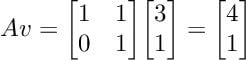
We can visualize the transformation of vector (v) with the following graph:

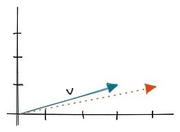
By looking at the example plot, we can see that the matrix-vector multiplication changed the vector’s direction. But what does this have to do with eigendecomposition?

It turns out when performing eigendecomposition, we are looking for a vector whose direction will not be changed by a matrix-vector multiplication. Only its magnitude will either be scaled up or down.

Therefore, the effect of the matrix on the vector is the same as the effect of a scalar on the vector.

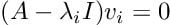
This effect can be described, more formally, by the fundamental eigenvalue equation:

After rearranging and factoring the vector (v) out, we get the following equation:

Now, we’ve arrived at the core idea of eigendecomposition. In order to find a non-trivial solution to the equation above, we first need to discover the scalars (λ) that shift the matrix (A) just enough to make sure a matrix-vector multiplication equals zero, sending the vector (v) in its null-space.

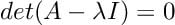
Thinking about it geometrically, we are looking for a matrix that squishes space into a lower dimension with an area or volume of zero. We can achieve this squishing effect when the matrix determinant equals zero.

The scalars (λ) we have to discover are called the eigenvalues, which unlock the calculation of the eigenvectors. We can envision the eigenvalues as some kind of keys unlocking the matrix to get access to the eigenvectors. But how do we find those keys?

How to Use Eigendecomposition to Find the Eigenvalues

As we briefly outlined in the previous section, we need to find the eigenvalues before we can unlock the eigenvectors.

An M x M matrix has M eigenvalues and M eigenvectors. Each eigenvalue has a related eigenvector, which is why they come in pairs. If we discover the eigenvalues, we hold the keys to unlock the associated eigenvectors.

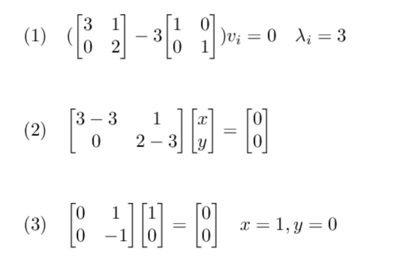
Imagine, we have a 2x2 matrix, and we want to compute the eigenvalues. By using the equation we derived earlier, we can calculate the characteristic polynomial and solve for the eigenvalues.

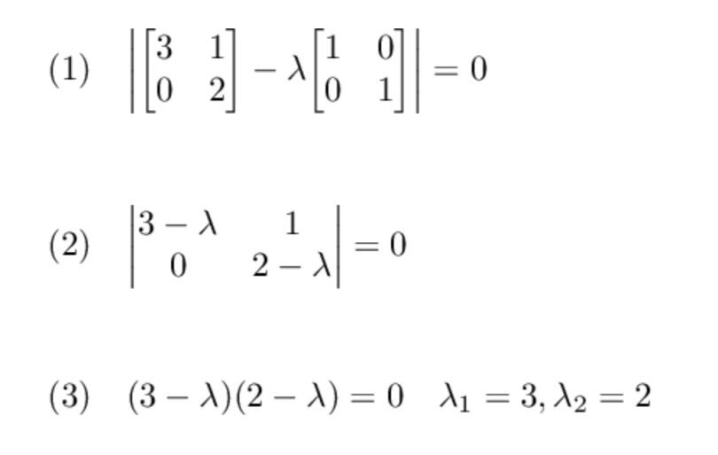
In our example, we just applied the formula (1), shifted the matrix by the eigenvalues (2), calculated the characteristic polynomial, and solved for the eigenvalues (3), which resulted in λ1=3 and λ2 = 2. Meaning the associated eigenvectors have a magnitude of three and two respectively.

Now, we can unlock the eigenvectors.

Finding the eigenvalues gets more involved and computationally expensive the larger the matrices become using the Abel-Ruffini theorem. Therefore, a whole family of iterative algorithms exists to compute the eigenvalues.

How to Use Eigendecomposition to Find the Eigenvectors

Eigenvectors describe the directions of a matrix and are invariant to rotations. Meaning the eigenvectors we are looking for will not change their direction.

We can use the eigenvalues, we discovered earlier, to reveal the eigenvectors.

Based on the fundamental eigenvalue equation, we simply pluck in the ith-eigenvalue and retrieve the ith-eigenvector from the null space of the matrix.

Let’s continue our example from before and use the already discovered eigenvalues λ1=3 and λ2 = 2, starting with λ1=3:

We inserted our first eigenvalue into the equation (1), shifted the matrix by that value (2) and finally solved for the eigenvector (3). The eigenvector for that unique eigenvalue λ1 is defined by x=1 and y=0.

The solution for the eigenvector, however, is not unique. We can imagine scaling the eigenvector by any scalar and still getting a valid result. There are basically an infinite amount of equally good solutions, which is the reason why we choose an eigenvector with unit norm,  a magnitude of one.

Continuing our example, we still need to solve for λ2 = 2. By applying the same steps as before, we retrieve our remaining eigenvector:

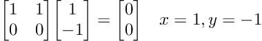
The eigenvector doesn’t have a length of one. To obtain an eigenvector with unit norm, we would have to scale it down by multiplying with 1/sqrt(2).

More on Data ScienceIntroduction to the Correlation Matrix

Eidgendecomposition and Matrix Reconstruction Example

Now that we know what eigendecomposition is and how to compute the eigenvalues and the eigenvectors, let’s work through a final example.

We will create a matrix, decompose and reconstruct it by using the built-in functions of NumPy. First, let’s create a simple 3x3 matrix and retrieve the eigenvalues and the eigenvectors.

# create simple 3x3 matrix
A = np.array([[10, 21, 36], [47, 51, 64], [72, 87, 91]])
# get eigenvalues and eigenvectors
values, vectors = np.linalg.eig(A)

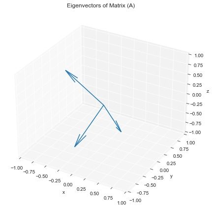
By running the code above we compute the eigenvalues and the eigenvectors. Since it’s in three dimensions, we can also try to visualize the eigenvectors.

# Eigenvalues
>> [170.53270055 -12.64773681  -5.88496373] 

# Eigenvectors
>>  [[-0.2509516  -0.87850736  0.71894055]
    [-0.53175418  0.22492691 -0.68983358]
    [-0.80886388  0.42146495  0.08517112]]

To reconstruct the original matrix (A), we can use the following equation:

We simply have to calculate the product of the eigenvectors, the eigenvalues and the inverse of the eigenvectors. Therefore, we need to diagonalize the eigenvalues and compute the inverse of the eigenvectors beforehand.

# diagonalize the eigenvalues
values = np.diag(values)
# invert the eigenvectors
vectors_inv = np.linalg.inv(vectors)
#reconstruct the original matrix
A_reconstructed = vectors @ values @ vectors_inv

print(A_reconstructed)

Printing the reconstructed matrix, we can see it contains the same values as our original matrix (A). Thus, we successfully reconstructed it.

# reconstructed matrix (A)
>>  [[10. 21. 36.]
    [47. 51. 64.]
    [72. 87. 91.]]

Eigendecomposition is a key element in the principal component analysis. The computation of the eigenvalues, however, is not as trivial as we have seen in our examples. Therefore, a plethora of iterative algorithms exists, to solve this particular problem.