What Is Pandas?

Pandas is a Python library for data analysis and data manipulation tasks. It works with many different types of data sets such as comma-separated values (CSV) files, Excel files, extensible markup language (XML) files, JavaScript object notation (JSON) files and relational database tables.

Wes McKinney created Pandas in 2008 and released it as an open-source project in 2010, thereby allowing anyone to contribute to its development. McKinney wrote Pandas on top of another Python library called NumPy that offers functionality such as n-dimensional arrays. 

There are several ways to get started with Pandas. You can install Python and Pandas locally or use an online Jupyter Notebook that allows you to write and execute Python in a web browser.

Data Structures in Pandas

Pandas has two main types of data structures: DataFrame and Series.

1. DataFrame

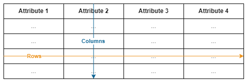
A DataFrame represents 2D tabular data containing labeled columns and rows with data (see figure 1 below). 

Pandas provide a lot of flexibility to work with DataFrame objects. For example, you can update the values of cells through various selecting methods, insert and delete rows, or remove duplicate rows. DataFrame objects can also be merged to combine data from multiple data sets, and plotting a chart of the data can often be reduced to a simple line of code.

2. Series

The Series object represents a 1D array of labeled data. The Series object is closely connected to the DataFrame object because the data of a column in a DataFrame is contained in a Series object. 

Both the Series and DataFrame objects contain, by default, a numerical sequence of numbers starting from zero and incrementing by one for each row. This is known as the Index. The Index can also be a sequence of strings or dates instead of numbers, and a Series object is therefore similar to the Python dictionary object in the sense it has a key for each value.

RelatedCreate the Classic Snake Game With Processing Library and Java

Advantages of Pandas

Functionality With Python

Pandas is available in a Python environment, thereby allowing us to implement it with many different Python functionality and APIs. 

Wide Variety of Pandas Methods

Whether or not you’d use Pandas over similar Python packages such as Vaex or Polars may depend on the specific use case and the readability of the API. For example, Pandas has a method to read data directly from a relational database that’s not currently offered by Vaex API.

Real-World Applications of Pandas

Pandas has a wide range of real-world applications related to data analysis, including everything from financial applications to scientific studies. 

Data Wrangling

Pandas can be used for data wrangling in order to transform data into a representation more suitable for analytics in different scenarios. Pandas offers features for data wrangling such as merging, sorting, cleaning, grouping and visualization. 

Descriptive Statistics

Pandas provides features to calculate descriptive statistics by allowing users to calculate a data set’s mean, standard deviation, quartiles, minimum and maximum. Pandas can also be combined with other Python packages such as SciPy to calculate inferential statistics, like ANOVA or paired sample t-tests.

Data Visualization

Pandas can implement another Python package called Matplotlib to create data visualizations like histograms, box plots and scatter plots.

RelatedA Guide to time Series Analysis in Python

How to Get Started With Pandas: A Tutorial

How to Install Pandas

Before installing Pandas locally, you have to ensure you’ve installed Python. Both Python and Pandas are supported on major operating systems such as Microsoft Windows, Apple macOS and Linux Ubuntu. If you haven’t installed Python yet, visit the Python website and find the distribution matching your current platform.

You can install Pandas with several different package manager tools such as pip or Anaconda. Before you do anything, I recommend reading the latest information about the different possibilities. 

That said, to install Pandas with pip simply enter the following into a terminal application:

$ pip install pandas

Start by importing Pandas with the alias pd by entering the following into a Python script:

​​​​​​​import pandas as pd

Pandas Data Structures

How to Create a Python Dictionary

To test out Pandas, you can create a simple dictionary object with some test data. For example, an object containing data about the number of seconds a list of runners spent to complete a run in seconds.

runners = {
 "name": [
 "Byron Hammond",
 "Lacey Austin",
 "Rebecca Bauer",
 "Yasir Burnett",
 "Clarence Rojas"
 ],
 "time": [120.2, 123.3, 133.6, 145.4, 160.2]
}

DataFrame in Pandas

After creating the test data, initialize a Pandas DataFrame object by calling pd.DataFrame with the data object as an argument:

df = pd.DataFrame(runners)

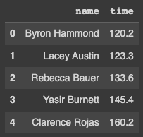
If you use Jupyter Notebook, you can simply output the DataFrame object by adding a line with the name of the variable at the bottom of the code block, and if you created a Python script where the code is outputted to a console, you have to print the variable using the following print method.

# Output the DataFrame in Jupyter Notebook
df

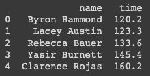
# Output the DataFrame in the console
print(df)

The console output of the DataFrame is very similar to the Jupyter Notebook output (see figures 2 and 3) below.

Series in Pandas

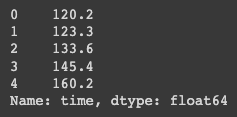
Each column of the DataFrame object is represented as a Series object. To get a specific column, insert the name of the column between square brackets after the name of the variable.

time = df["time"]

As you can see in figure 4, the Series object is a list with the time information wherein each row has an index like the DataFrame object.

Pandas DataFrame Methods

Head() in Pandas

Pandas provides a method called head() you can use to output the beginning of a DataFrame or a Series object.

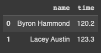
df.head(2)

You can pass an integer to the method to define the number of rows you want to return. If no integer is passed, the default number of rows is automatically set to five. You can see in figure 5 below that the method returns the rows with indexes 0 and 1.

Tail() in Pandas

Pandas also provides another method called tail() you can use to output the ending of a DataFrame or a Series object.

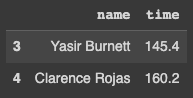
df.tail(2)

As with the method head(), you can pass an integer to define the number of rows, and the default number is five. Figure 6 shows the method returns the rows with indexes three and four.

Loc() in Pandas

Pandas provides many different ways to get data from a DataFrame or Series object. For example, another method is to use boolean operations by calling the method loc().

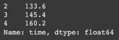
time2 = df.loc[(df["time"] > 130), "time"]

You can see in figure 7 that the method returns a Series object containing the last three runners because their time property is greater than 130.

Pandas Statistical and Data Visualization Methods  

Describe() in Pandas

To calculate a descriptive statistic for a DataFrame or Series object, use the method describe().

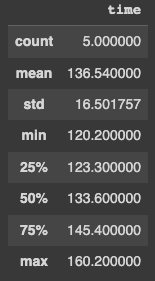
df.describe()

You can see in figure 8 that the method returns the number of runners (count), the mean, standard deviation (std), minimum and maximum, and the three quartiles (25 percent, 50 percent and 75 percent).

Boxplot() in Pandas

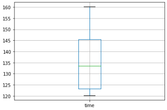
You can use the boxplot() method to visualize the statistical data returned by the describe() method.

df.boxplot()

In figure 9, you can see that Pandas returns a box plot over the data.

Data_Range() and Corr() in Pandas

You can also use Pandas to calculate the correlation between multiple data sets by using corr(). First, create some test data by creating a range of dates using the method date_range() and define an object containing the price of two different stocks.

dates = pd.date_range('1/1/2022', periods=8)
stocks = {
 "stock1": [104, 113, 114, 115, 120, 116, 123, 125],
 "stock2": [101, 104, 109, 103, 113, 116, 111, 114]
}

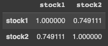
Next, initialize the DataFrame object and call the method corr(). Notice that the DataFrame object initializes using both the data object and an index (instead of only the data object as in the earlier example) to specify each row is identified by a date. The dates are not important for the method corr() but will be convenient later when plotting the two stocks’ graphs.

df = pd.DataFrame(stocks, index=dates)
df.corr()

The method corr() returns the Pearson correlation coefficient by default but it’s possible to use the Kendall rank correlation coefficient or Spearman’s rank correlation coefficient by passing either kendall or spearman as an argument. As you can see in figure 10, the correlation coefficient between stock1 and stock2 is 0.7.

Heatmap() in Pandas

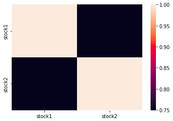
Another way to visualize the result of corr() is to display a heatmap. You can do this quite easily by combining the Pandas DataFrame object with another Python package called Seaborn. Import the package as sns and call the method heatmap() with the correlation matrix as an argument.

import seaborn as sns
sns.heatmap(df.corr())

As you can see in figure 11, the method heatmap() returns a heatmap over the different values in the correlation matrix.

Plot() in Pandas

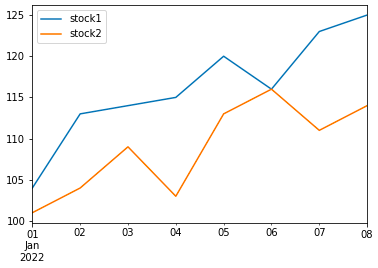
Finally, Pandas has a method called plot() that you can use to see a simple line graph over the two stock prices.

df.plot()

You can see in the figure below that Pandas output a graph where the x-axis specifies the DataFrame object’s indexes and the y-axis specifies the stocks’ prices. 

As shown in the examples above, you can easily use Pandas DataFrame and Series objects to analyze many types of data sets. However, the examples only show a few of the possibilities that Pandas has to offer and you might want to look into other use cases, such as how to use Pandas’ group by functionality or how to handle missing data.

Alternatives to Pandas

There are many analytics tools that have very similar functionality to Pandas, whether you are looking for a traditional GUI-based tool, another Python package, or a tool written in another programming language, it’s possible to find a suitable alternative. 

Polars and Vaex Libraries

Examples of similar Python packages to Pandas are Polars and Vaex. Both are faster than Pandas at some operations when working with larger data sets, and offer similar functionality such as DataFrame objects, import/export CSV and aggregations methods. Both packages also support creating DataFrame objects from Pandas DataFrame objects.

Microsoft Excel and Google Sheets

Traditional GUI-based spreadsheet software such as Microsoft Excel and Google Sheets both contain methods to handle tabular data, import/export CSV, calculate different aggregation methods such as mean or average, and have the ability to visualize data like in Pandas. 

Aquero (JavaScript), Rover (Ruby) and R

For Pandas alternatives in other programming languages, the JavaScript library Arquero, the Ruby library Rover or the programming language R might suit your needs. All three alternatives offer DataFrame object functionality to work with tabular data.

Frequently Asked Questions