The Dirichlet Distribution: What Is It and Why Is It Useful?

If you look up the Dirichlet distribution in any textbook, you’ll encounter the following definition:

An immediate question is why do we use the Dirichlet distribution as a prior distribution in Bayesian statistics? One reason is that it’s the conjugate prior to two important probability distributions: the categorical distribution and the multinomial distribution. In short, using the Dirichlet distribution as a prior makes the math a lot easier.

More on Data Science4 Probability Distributions Every Data Scientist Needs to Know

Conjugate Prior

In Bayesian probability theory, if the posterior distribution p(θ|x) and the prior distribution p(θ) are from the same probability distribution family, then the prior and posterior are called conjugate distributions, and the prior is the conjugate prior for the likelihood function.

If we think about the problem of inferring the parameter θ for a distribution from a given set of data x, then Bayes’ theorem says the posterior distribution is equal to the product of the likelihood function θ → p(x|θ) and the prior p(θ), normalized by the probability of the data p(x):

Since the likelihood function is usually defined from the data generating process, the difference choices of prior can make the integral more or less difficult to calculate. If the prior has the same algebraic form as the likelihood, then often we can obtain a closed-form expression for the posterior, avoiding the need of numerical integration.

More on Data Science5 Open-Source Machine Learning Libraries Worth Checking Out

Motivating the Dirichlet Distribution

Here’s how the Dirichlet distribution can be used to characterize the random variability of a multinomial distribution. I’ve borrowed this example from a great blog post on visualizing the Dirichlet distribution.

Suppose we’re going to manufacture six-sided dice but allow the outcomes of a toss to be only one, two or three (so the later visualization is easier). If the die is fair then the probabilities of the three outcomes will be the same and equal to 1/3. We can represent the probabilities for the outcomes as a vector θ =(θ₁, θ₂, θ₃).

θ has two important properties: First, the sum of the probabilities for each entry must equal one, and none of the probabilities can be negative. When these conditions hold, we can use a multinomial distribution to describe the results associated with rolling the die.

In other words, if we observe n dice rolls, D={x₁,…,x_k}, then the likelihood function has the form:

Where N_k is the number of times the valuek∈{1, 2, 3} has occurred.

We expect there will be some variability in the characteristics of the dice we produce, so even if we try to produce fair dice, we won’t expect the probabilities of each outcome for a particular die will be exactly 1/3, due to variability in the production process. To characterize this variability mathematically, we would like to know the probability density of every possible value of θ for a given manufacturing process. To do this, let’s consider each element of θ as being an independent variable.

That is, for θ =(θ₁, θ₂, θ₃), we can treat θ₁, θ₂ and θ₃ each as an independent variable. Since the multinomial distribution requires that these three variables sum to one, we know that the allowable values of θ are confined to a plane. Furthermore, since each value θᵢ must be greater than or equal to zero, the set of all allowable values of θ is confined to a triangle.

What we want to know is the probability density at each point on this triangle. This is where the Dirichlet distribution can help us: We can use it as the prior for the multinomial distribution.

Built In Machine Learning TutorialsA Step-by-Step NLP Machine Learning Classifier Tutorial

Dirichlet Distribution

The Dirichlet distribution defines a probability density for a vector valued input having the same characteristics as our multinomial parameter θ. It has support (the set of points where it has non-zero values) over:

K is the number of variables. Its probability density function has the following form:

The Dirichlet distribution is parameterized by the vector α, which has the same number of elements K as our multinomial parameter θ. So you can interpret p(θ|α) as the answer to the question “what is the probability density associated with multinomial distribution θ, given that our Dirichlet distribution has parameter α?”

More on Data ScienceThe Poisson Process and Poisson Distribution, Explained

Visualizing the Dirichlet Distribution

We see the Dirichlet distribution indeed has the same form as the multinomial likelihood distribution. But what does it actually look like?

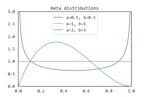
To see this, we need to note that the Dirichlet distribution is the multivariate generalization of the beta distribution. The beta distribution is defined on the interval [0, 1] parameterized by two positive shape parameters α and β. As you might expect, it is the conjugate prior of the binomial (including Bernoulli) distribution. The figure shows the probability density function for the Beta distribution with a few α and β values.

As we can see, the beta density function can take a wide variety of different shapes depending on α and β. When both α and β are less than one, the distribution is U-shaped. In the limit of α = β → 0, it is a  two point Bernoulli distribution with equal probability 1/2 at each Dirac delta function ends x=0 and x=1, and zero probability everywhere else. When α=β=1 we have the uniform [0, 1] distribution, which is the distribution with the largest entropy. When both α and β are greater than one the distribution is unimodal. This diversity of shapes by varying only two parameters makes it particularly useful for modeling actual measurements.

For the Dirichlet distribution Dir(α) we generalize these shapes to a K simplex. For K=3, visualizing the distribution requires us to do the following: 

1. Generate a set of x-y coordinates over our triangle 
2. Map the x-y coordinates to the two-simplex coordinate space
3. Compute Dir(α) for each point 

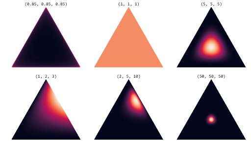
Below are some examples, you can find the code in my Github repository.

We see it’s now the parameter α that governs the shapes of the distribution. In particular, the sum α₀=∑αᵢ controls the strength of the distribution (how peaked it is). If αᵢ < 1 for all i, we get spikes at the corners of the simplex. For values of αᵢ > 1, the distribution tends toward the centre of the simplex. As α₀ increases, the distribution becomes more tightly concentrated around the centre of the simplex.

In the context of our original dice experiment, we would produce consistently fair dice as αᵢ → ∞. For a symmetric Dirichlet distribution with αᵢ > 1, we will produce fair dice, on average. If the goal is to produce loaded dice (e.g., with a higher probability of rolling a three), we would want an asymmetric Dirichlet distribution with a higher value for α₃.

Now you’ve seen what the Dirichlet distribution looks like, and the implications of using it as a prior for a multinomial likelihood function in the context of dice manufacturing. 

Frequently Asked Questions